NURBS-Warps
This section introduces a new warp, the NURBS-Warp, which is built upon tensor-product Non-Uniform Cubic B-Splines.
We show that the NURBS-Warp naturally appears when replacing the affine projection by a perspective one in the image formation model of the previous section.
As our experimental results will show, the NURBS-Warp performs better in the presence of perspective effects.
All the necessary details about the NURBS model have been presented in section 2.3.3.
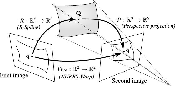
Following the same reasoning than for the BS-Warp in the previous section, we show that the NURBS-Warp corresponds to perspective imaging conditions.
This is illustrated in figure 6.3.
Figure 6.3:
A NURBS-Warp can be seen as the result of a threedimensional B-Spline surface projected under perspective conditions.
|
 |
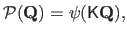
Let
 be the perspective projection:
 |
(6.8) |
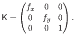
with
 the matrix of intrinsic parameters for the second camera.
 is the homogeneous to affine coordinates function, i.e.
 where
where
 are the homogeneous coordinates of
 (
(
 ).
We assume that the image coordinates are chosen such that the origin coincides with the principal point:
).
We assume that the image coordinates are chosen such that the origin coincides with the principal point:
 |
(6.9) |
Replacing
 by its expression of equation (6.3) in equation (6.8) leads to:
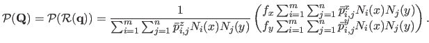 |
(6.10) |
Defining
 ,
,
 and
and
 , equation (6.10) is the very definition of a tensor-product NURBS with control points
 and weights
  (see section 2.3.3).
We denote
(see section 2.3.3).
We denote
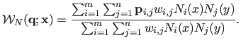
 this new warp and call it a NURBS-Warp:
 |
(6.11) |
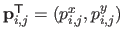
Here, the warp parameters, i.e. the control points and the weights, are grouped into a vector
 .
.
Using the NURBS-Warp in the setup used for the experiment of figure 6.2 leads to a transfer error consistently smaller than  pixels.
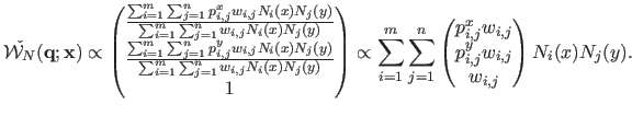
The NURBS-Warp defined by equation (6.11) can be expressed with homogeneous coordinates.
We note
 the NURBS-Warp in homogeneous coordinates:
 |
(6.12) |
We observe that in the homogeneous version of equation (6.12), our NURBS-Warp does a linear combination of control points in homogeneous coordinates, as opposed to the classical BS-Warp of equation (6.2) that does a linear combination of control points in affine coordinates.
This is what makes our NURBS-Warp able to model perspective projection, thanks to the division `hidden' in the homogeneous coordinates.
Contributions to Parametric Image Registration and 3D Surface Reconstruction (Ph.D. dissertation, November 2010) - Florent Brunet
Webpage generated on July 2011
PDF version (11 Mo)