Affine Interpretation of the BS-Warps
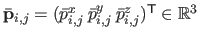
In this chapter, we denote
 the BS-Warp.
As a reminder of section 2.3.2, a BS-Warp is defined as:
the BS-Warp.
As a reminder of section 2.3.2, a BS-Warp is defined as:
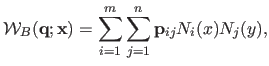 |
(6.2) |
where the functions
 are the B-Spline basis functions and the
 are the control points (grouped in the parameter vector
 ).
The scalars
).
The scalars  and
and  are the number of control points along the
  and
and  directions respectively.
Note that we consider as coincident the knot sequences used to define the B-Spline basis functions.
directions respectively.
Note that we consider as coincident the knot sequences used to define the B-Spline basis functions.
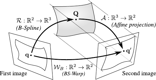
If we consider that the observed surface is modelled by a threedimensional tensor-product B-Spline, the BS-Warp corresponds to the transformation between the two images under affine imaging conditions (see figure 6.1 for an illustration).
Figure 6.1:
A BS-Warp can be seen as the result of a threedimensional B-Spline surface projected under affine conditions.
|
 |
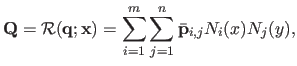
Let
 be the 2D-3D map between the first image and the threedimensional surface:
 |
(6.3) |
with
 the 3D control points of the surface.
Let
the 3D control points of the surface.
Let
 be the affine projection of the surface into the second image:
 |
(6.4) |
with
 the matrix which models the affine projection, assuming that the 3D surface is expressed within the coordinate frame of the second camera:
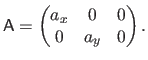 |
(6.5) |
Given these notations, the warped point
 can be written
 which, after expansion, gives:
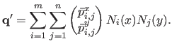 |
(6.6) |
Equation (6.6) matches the definition of equation (6.2) of a BS-Warp.
As we just demonstrated, BS-Warps are obtained under affine imaging conditions.
However, this does not prove that they are not suited for perspective imaging conditions.
In this paragraph, we experimentally illustrate that BS-Warps are indeed not suited for perspective imaging conditions.
This comes from the fact that the division appearing in a perspective projection is not present in the BS-Warp model.
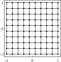
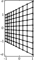
The bad behavior of the BS-Warp in the presence of perspective effects is illustrated in figure 6.2.
In this experiment, we simulate a set of point correspondences by transforming a regular grid with an homography parametrized by a scalar  that controls the amount of perspective effect.
The
that controls the amount of perspective effect.
The
 matrix of this homography,
 , is given by:
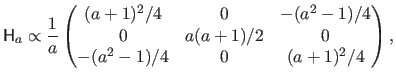 |
(6.7) |
where  indicates equality up to scale.
The larger
indicates equality up to scale.
The larger  , the more important the perspective effect.
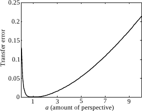
Figure 6.2 c clearly shows that the transformation can be correctly modelled by a BS-Warp only when
, the more important the perspective effect.
Figure 6.2 c clearly shows that the transformation can be correctly modelled by a BS-Warp only when  , i.e. when the perspective effect is barely existant.
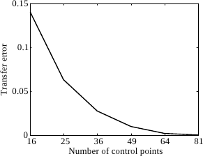
Figure 6.2 d shows that the number of control points of a BS-Warp must be significantly large in order to correctly model a perspective effect.
, i.e. when the perspective effect is barely existant.
Figure 6.2 d shows that the number of control points of a BS-Warp must be significantly large in order to correctly model a perspective effect.
Figure 6.2:
Bad behavior of the BS-Warp in the presence of perspective effects. (a) Data points on a regular grid (first image). (b) Transformed points simulating a perspective effect with an homography (second image). (c) Influence of the perspective effect on a BS-Warp with 16 control points. (d) The perspective effect (
 ) can be modeled with a BS-Warp but it requires a large amount of control points.
|
|
Contributions to Parametric Image Registration and 3D Surface Reconstruction (Ph.D. dissertation, November 2010) - Florent Brunet
Webpage generated on July 2011
PDF version (11 Mo)