Subsections
Smooth and Inextensible Surface Reconstruction
Although the strategem of maximizing the sum of depths
 described in the previous section gives reasonable results, it is merely
a heuristic, not based on any valid principle related to surface properties.
We therefore consider next a new formulation based on the principle
of surface inextensibility.
described in the previous section gives reasonable results, it is merely
a heuristic, not based on any valid principle related to surface properties.
We therefore consider next a new formulation based on the principle
of surface inextensibility.
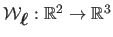
Let the surface be modelled as a function
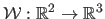 ,
mapping the planar template to
,
mapping the planar template to  -dimensional space.
The inextensibility constraint is equivalent to saying
that the map
-dimensional space.
The inextensibility constraint is equivalent to saying
that the map
 must be everywhere a local isometry. This condition
may be expressed in terms of its Jacobian.
Let
must be everywhere a local isometry. This condition
may be expressed in terms of its Jacobian.
Let
 be the Jacobian matrix
 evaluated at the point
 .
The map
is an isometry at
if the columns of
.
The map
is an isometry at
if the columns of
 are
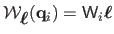
orthonormal. This local isometry can be enforced for the whole surface with
the following least-squares constraint:
are
orthonormal. This local isometry can be enforced for the whole surface with
the following least-squares constraint:
 |
(7.7) |
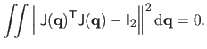
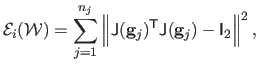
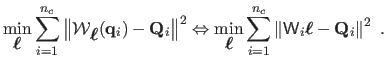
In practice, we consider a discretization of the quantity in
equation (7.7), namely
 |
(7.8) |
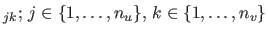
where
 is a set of 2D points in the template image
space taken on a fine and regular grid (for instance, a grid of size
is a set of 2D points in the template image
space taken on a fine and regular grid (for instance, a grid of size
 ). This term
 measures the departure from
inextensibility of the surface
.
measures the departure from
inextensibility of the surface
.
Our minimization problem is then to minimize this quantity, over all
possible surfaces, subject to the projection constraints,
namely that point
 projects to (or near to) the image
point
projects to (or near to) the image
point
 , for all
  .
.
The problem just described involves a minimization over all possible
surfaces. Instead of considering this as a variational problem over
all possible surfaces, we consider a parametrized family of
surfaces. For this purpose, we chose Free-Form Deformations
(FFD) (162) based on uniform cubic B-splines (61).
All the details on this parametric model have been given in section 2.3.2.
Here, we just precise the notation used in this chapter.
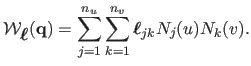
Let
 be the parametric FFD,
parametrized by a family of 3D points
be the parametric FFD,
parametrized by a family of 3D points

 , which act
as `attractors' for the surface.
, which act
as `attractors' for the surface.
For a point
 in the template, the surface point
is explicitly given as
in the template, the surface point
is explicitly given as
 |
(7.9) |
The functions  are the B-spline basis functions (61)
which are polynomials of degree . If point
are the B-spline basis functions (61)
which are polynomials of degree . If point
 is fixed and known then the surface point
 is expressed as a linear combination of the points
 ,
and hence can be written in the form
,
and hence can be written in the form
 , where
 is a
is a
 matrix depending only on the point
 ,
and
is the vector obtained by concatenating all the points
. Thus, the 3D point is a linear expression in terms of the
parameter vector
.
Since the polynomials and
,
and
is the vector obtained by concatenating all the points
. Thus, the 3D point is a linear expression in terms of the
parameter vector
.
Since the polynomials and  depend only on a local set of the attractor points
,
the matrix
is sparse, which is important for computational efficiency.
depend only on a local set of the attractor points
,
the matrix
is sparse, which is important for computational efficiency.
Surface Reconstruction as a Least-Squares Problem
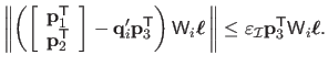
By replacing
 by
in equation (7.6)
we may arrive at a constraint:
by
in equation (7.6)
we may arrive at a constraint:
 |
(7.10) |
We may then formulate the optimization problem as
minimizing the inextensibility cost
 given in equation (7.8)
over all choices of parameters
, subject to constraints
equation (7.10). The constraints are SOCP constraints,
but the cost function equation (7.8) is of
higher degree in the parameters. To avoid the difficulties of constrained
non-linear optimization, we choose a different course, by
including the reprojection error into the cost function, leading to
an unconstrained problem.
given in equation (7.8)
over all choices of parameters
, subject to constraints
equation (7.10). The constraints are SOCP constraints,
but the cost function equation (7.8) is of
higher degree in the parameters. To avoid the difficulties of constrained
non-linear optimization, we choose a different course, by
including the reprojection error into the cost function, leading to
an unconstrained problem.
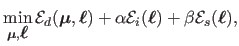
To simplify the formulation of the reprojection error, we introduce
the depths  as subsidiary variables, for reasons that become
evident below. This is not strictly necessary, but reduces the degree
of the reprojection-error term. The minimization problem now takes the form:
as subsidiary variables, for reasons that become
evident below. This is not strictly necessary, but reduces the degree
of the reprojection-error term. The minimization problem now takes the form:
 |
(7.11) |
where
 ,
,
 ,
,
 are the data (reprojection error),
inextensibilty, and smoothing terms respectively.
The data term ensures the consistency of the point correspondences with the
reconstructed surface.
forces the inextensibility of the surface.
are the data (reprojection error),
inextensibilty, and smoothing terms respectively.
The data term ensures the consistency of the point correspondences with the
reconstructed surface.
forces the inextensibility of the surface.
 promotes smooth surface in order to cope with, for instance, lack
of data.
The relative influence of these three terms are controlled with the
weights
promotes smooth surface in order to cope with, for instance, lack
of data.
The relative influence of these three terms are controlled with the
weights
 and
and
 .
Note that the choice of
.
Note that the choice of  and
and  is generally not critical.
The inextensibility term has been described previously. We now describe
the two other terms in equation (7.11).
Replacing
by
in equation (7.5)
gives an expression for the reprojection error associated with some point.
However, the resulting expression is non-linear with respect to the
parameters
.
We thus prefer a linear data term expressed in terms of `3D errors', which
is the reason why we introduced the depths
 of the data points in
the optimization problem.
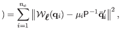
The data term is then defined by:
of the data points in
the optimization problem.
The data term is then defined by:
which measures the distance between the point
 on the surface
and the point at depth along the ray defined by
.
on the surface
and the point at depth along the ray defined by
.
In some cases, the point correspondences and the hypothesis of an
inextensible surface are not sufficient.
For instance, imagine that there is no point correspondence in a corner of
the surface.
In this case, there is nothing that indicates how the surface should behave.
The corners of the surface can bend freely as long as they do not extend or
shrink (like the corners of a piece of paper).
To overcome this difficulty, we can add a third term (the smoothing term)
in our cost function that favours non-bending surfaces.
Note that usually, such terms are used to compensate for the undesirable
effects of under-fitting and over-fitting.
Doing so is usually a problem because it requires one to determine a correct
value for the weight associated to the smoothing term (value in
equation (7.11)).
This is a sensible and critical way of balancing the effective complexity
of the surface against the complexity of the data.
Here, we do not have to care too much.
Indeed, the complexity of the surface is limited by the fact
that it is inextensible.
Any small value (but big enough to be not negligible, for instance
 ) is thus suitable for the weight of the smoothing term.
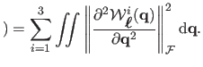
We define our smoothing term using the bending energy:
) is thus suitable for the weight of the smoothing term.
We define our smoothing term using the bending energy:
where
 is the -th coordinate of the
point, and
is the -th coordinate of the
point, and
 is the Frobenius norm of the Hessian matrix.
With FFD, there exists a simple and linear closed-form expression for the
bending energy:
is the Frobenius norm of the Hessian matrix.
With FFD, there exists a simple and linear closed-form expression for the
bending energy:
where
 is a symmetric, positive, and semi-definite
matrix which can be easily computed from the second derivatives of the
B-spline basis functions.
is a symmetric, positive, and semi-definite
matrix which can be easily computed from the second derivatives of the
B-spline basis functions.
The problem of equation (7.11) is a non-linear least-squares
minimization problem typically solved using an iterative scheme such as
Levenberg-Marquardt.
Such an algorithm requires a correct initial solution.
We used an FFD surface fitted to the 3D points reconstructed with
one of the point-wise methods presented in section 7.3.
Subsequently, since we use a surface model which is linear with respect to its
parameters, the initial parameters
can be found by solving the
least-squares problem:
 |
(7.15) |
An alternative is to modify the problem (7.6),
expressing
in terms of
the required parameters
, according to
 .
Then one may solve for
directly using SOCP.
If necessary, the linear smoothing term of equation (7.13) can
be included in equation (7.15).
.
Then one may solve for
directly using SOCP.
If necessary, the linear smoothing term of equation (7.13) can
be included in equation (7.15).
Contributions to Parametric Image Registration and 3D Surface Reconstruction (Ph.D. dissertation, November 2010) - Florent Brunet
Webpage generated on July 2011
PDF version (11 Mo)