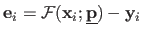
BleamCard: the first augmented reality card. Get your own on Indiegogo!
Subsections
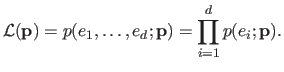
Parameter Estimation
The vast majority of the problems treated in this document reduces to parameter estimation problems.
In this section, we give the basic tools and concepts related to such problems.
Broadly speaking, the goal of parameter estimation is to estimate (or infer) the unknown parameters of a fixed model in order to fit some noisy measurements.
It relies on an analysis of the probability density functions of the error in the measurements.
This section is organized as follows.
We first give some general points on parameter estimation.
We then give some specializations of the general points.
General Points on Parameter Estimation
Parametric Models of Function
The first thing to do in a parameter estimation problem is to choose a parametric model of function.
Note that in this document the expression `parametric model of function' will often be abbreviated to `parametric model' or even `model'.
A parametric model is a family of functions that can be described with a finite set of parameters.
These parameters are generally grouped in a vector
 .
The parametric model is the following family of functions:
.
The parametric model is the following family of functions:
 |
(3.1) |
We generally designate a parametric model with the notation
 .
A standard convention is to note
.
A standard convention is to note
 a particular element of the parametric model (for a given set of parameters
 ).
We do not follow this convention in this document.
This stems from the fact that we sometimes want to consider the function
).
We do not follow this convention in this document.
This stems from the fact that we sometimes want to consider the function
 as a function of its natural parameters for a fixed set of parameters
(i.e. the function
as a function of its natural parameters for a fixed set of parameters
(i.e. the function
 ).
Some other times we consider
as a function of the parameters for a given set of natural parameters
).
Some other times we consider
as a function of the parameters for a given set of natural parameters
 (i.e. the function
 ).
).
The choice of the model depends mainly on the hypothesis we are able to make on the data to fit.
For instance, if one wanted to study the motion of a ball thrown by a basketball player, a good model may be a polynomial of degree 2.
The most used models in this thesis have been detailed in section 2.3.
The goal of parameter estimation is to determine a set of parameters
so that the resulting function
 is close to the data measurements.
From now on and without any loss of generality, we assume that the model is made of scalar-valued functions.
The data points, i.e. the measurements, can be seen as noisy instances of a reference function
 .
Let us note
.
Let us note
 the set of the
  measurements with
 and
and
 .
We have that:
.
We have that:
 |
(3.2) |
where
 is a random variable.
Estimation techniques relies on an analysis of the errors
.
In particular, an estimation technique depends on the probability distribution assumed for the random variables
.
is a random variable.
Estimation techniques relies on an analysis of the errors
.
In particular, an estimation technique depends on the probability distribution assumed for the random variables
.
Let  be a continuous random variable.
The probability density function
be a continuous random variable.
The probability density function  of the random variable is a function from
 to
to
 such that:
![$\displaystyle P [ a \leq X \leq b ] = \int_a^b p(x) \mathrm d x,$](img576.png) |
(3.3) |
where
![$ P [ a \leq X \leq b ]$](img577.png) denotes the probability that lies in the interval
denotes the probability that lies in the interval ![$ [a,b]$](img63.png) .
In order to be a PDF, a function must satisfy several criteria.
First, it must be a positive function.
Second, it must be integrable.
Third, it must satisfies:
.
In order to be a PDF, a function must satisfy several criteria.
First, it must be a positive function.
Second, it must be integrable.
Third, it must satisfies:
 |
(3.4) |
The PDF of a random variable defines the distribution of that variable.
Some common distributions (and what they imply in terms of parameter estimation) will be detailed later in this section.
The cumulative distribution function  associated to the PDF is the function from
to
defined by:
associated to the PDF is the function from
to
defined by:
 |
(3.5) |
Note that since is a positive function, is an increasing function.
Maximum Likelihood Estimation (MLE) is a statistical tool used to find the parameters of a model given a set of data.
The general idea behind MLE is to find the `most probable' parameters
given the observations.
Let
be the observations.
Let  be the residual3.1 for the
  -th data point for a given set of parameters
, i.e.
-th data point for a given set of parameters
, i.e.
 .
Note that depends on the parameters
even though this dependency is not explicitly written.
We consider the residuals as random variables.
Let us assume that the variables are independent and identically distributed (i.i.d.).
This allows us to say that the joint probability of the variables
.
Note that depends on the parameters
even though this dependency is not explicitly written.
We consider the residuals as random variables.
Let us assume that the variables are independent and identically distributed (i.i.d.).
This allows us to say that the joint probability of the variables
 given the model parameters
is:
given the model parameters
is:
![$\displaystyle P[e_1, \ldots, e_d \vert \mathbf{p}] = \prod_{i=1}^d P[e_i \vert \mathbf{p}],$](img584.png) |
(3.6) |
where ![$ P[A \vert B]$](img585.png) denotes the probability of the event
denotes the probability of the event  given the event
  and
and
![$ P[A_1, \ldots, A_n]$](img586.png) denotes the joint probability of the events
denotes the joint probability of the events
 .
In terms of probability density function, it means that we have:
.
In terms of probability density function, it means that we have:
 |
(3.7) |
where is the probability density function associated to the distribution of the random variables .
The likelihood function
 is the joint probability density function considered as a function of the parameters
:
is the joint probability density function considered as a function of the parameters
:
 |
(3.8) |
MLE amounts to maximize the likelihood of the parameters
, i.e.:
 |
(3.9) |
From a practical point of view, it is often more convenient to consider the log-likelihood instead of the likelihood.
The log-likelihood
 is the function defined as:
 |
(3.10) |
In this way, equation (3.9), which is a maximization problem with a cost function defined as a product of numerous factors, can easily be turned into a minimization problem with a cost function defined as a simple sum:
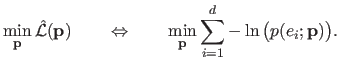 |
(3.11) |
MLE will be instantiated to specific distributions later in this section.
For now, let us just say that least-squares problems are the natural consequence of MLE with normally-distributed errors.
Maximum A Posteriori Estimation
For MLE, we specified a distribution
 for the residuals given the parameters
.
For the method of Maximum a Posteriori (MAP), we also specify a prior distribution
for the residuals given the parameters
.
For the method of Maximum a Posteriori (MAP), we also specify a prior distribution
 on the parameters
that reflects our knowledge about the parameters independently of any observation (96).
As an example of parameter prior, one may assume that the fitted function must be `smooth'.
The posterior distribution
on the parameters
that reflects our knowledge about the parameters independently of any observation (96).
As an example of parameter prior, one may assume that the fitted function must be `smooth'.
The posterior distribution
 is then computed using the Bayes rule:
 |
(3.12) |
The denominator in the right hand side of equation (3.12) acts as a normalizing constant chosen such that
is an actual probability density function.
The MAP estimation method amounts to solve the following maximization problem:
 |
(3.13) |
Note that MAP is equivalent to MLE if the prior distribution of the parameters
is chosen to be a uniform distribution.
In this case, we say that we have an uninformative prior.
An estimator is a function that maps a set of observations to an estimate of the parameters.
In other words, an estimator is the result of an estimation process and of a model applied to a set of data.
If
are the parameters we wish to estimate, then the estimator of
is typically written by adding the `hat' symbol:
 .
The notion of estimator is independent of any particular model or estimation process.
In particular, it may not be formulated as an optimization problem.
This is the reason why the generic notation
is used.
Note that, by abuse of language,
designates either the estimator itself or the estimated parameters.
.
The notion of estimator is independent of any particular model or estimation process.
In particular, it may not be formulated as an optimization problem.
This is the reason why the generic notation
is used.
Note that, by abuse of language,
designates either the estimator itself or the estimated parameters.
The bias of an estimator is the average error between estimations
and the corresponding true parameters
 (for a given set of data).
Let
(for a given set of data).
Let
 be the residuals associated to the estimated model, i.e.
 .
The bias is formally defined as (95):
.
The bias is formally defined as (95):
![$\displaystyle E[\hat{\mathbf{p}} ; \underline{\mathbf{p}}, \mathbf{e}] - \under...
...{\mathbf{p}}) \hat{\mathbf{p}} \;\mathrm d \mathbf{e} - \underline{\mathbf{p}},$](img604.png) |
(3.14) |
where
![$ E[\hat{\mathbf{p}} ; \underline{\mathbf{p}}, \mathbf{e}]$](img605.png) is the expectation of having the estimate
knowing the true parameters
and the errors
is the expectation of having the estimate
knowing the true parameters
and the errors
 .
Another way to explain the bias of an estimator is to consider a given set of parameters
.
Then an experiment is repeated with the same parameters
but with different instance of the noise at each trial.
The bias is the difference between the average value of the estimated parameters
and the true parameters
.
.
Another way to explain the bias of an estimator is to consider a given set of parameters
.
Then an experiment is repeated with the same parameters
but with different instance of the noise at each trial.
The bias is the difference between the average value of the estimated parameters
and the true parameters
.
A desirable property for an estimator is to be unbiased.
This means that on average with an infinite set of data, there is no difference between the estimated model
and the corresponding true model
.
Another important property of an estimator is its variance.
Imagine an experiment repeated many times with the same parameters
but with different instance of the noise at each trial.
The variance of the estimator is the variance of the estimated parameters
.
In case where
is a vector, we talk about the covariance matrix instead of the variance.
It is formally defined as:
![$\displaystyle \mathrm{Var}[\hat{\mathbf{p}} ; \underline{\mathbf{p}} , \mathbf{...
... \underline{\mathbf{p}}, \mathbf{e}])^2 ; \underline{\mathbf{p}} , \mathbf{e}].$](img607.png) |
(3.15) |
A low variance means that a change in the instance of noise have little effect on the estimated parameters
.
The variance of an estimator is sometimes called its efficiency.
For an estimator, it is a desirable property to be efficient, i.e. have a low variance.
In other words, its preferable that the noise does not affect too much an estimator.
Usually, we are more interested in the Mean-Squared Residual (MSR) of an estimator than in its variance.
The MSR measures the average error of the estimated parameters with respect to the true parameters.
It is formally defined as:
![$\displaystyle MSR[\hat{\mathbf{p}} ; \underline{\mathbf{p}} , \mathbf{e}] = E[(...
...\mathbf{p}} - \underline{\mathbf{p}})^2 ; \underline{\mathbf{p}} , \mathbf{e}].$](img608.png) |
(3.16) |
The variance, the bias and the MSR of an estimator are linked with the following relation:
![$\displaystyle MSR[\hat{\mathbf{p}} ; \underline{\mathbf{p}} , \mathbf{e}] = \ma...
...{\mathbf{p}} ; \underline{\mathbf{p}}, \mathbf{e}] - \underline{\mathbf{p}})^2.$](img609.png) |
(3.17) |
Note that the rightmost term in equation (3.17) is the squared bias of the estimator.
In this section we specify some classical estimators that derives from particular assumptions on the distribution of the noise.
We will also give the properties of these estimators.
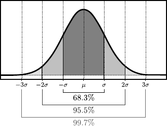
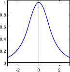
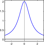
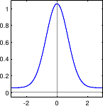
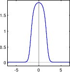
Normal Distribution and Least-Squares
The normal distribution, also known as the Gaussian distribution, is a continuous probability distribution used to describe a random variable that concentrates around its mean.
This distribution is parametrized by two parameters: the mean
 , and the standard deviation
 .
The normal distribution with parameters
.
The normal distribution with parameters  and
and  is denoted
 .
Table 3.1 gives the main properties of
.
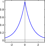
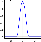
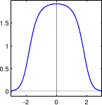
Figure 3.1 illustrates the PDF of the normal distribution.
.
Table 3.1 gives the main properties of
.
Figure 3.1 illustrates the PDF of the normal distribution.
The multivariate normal distribution is a generalization of the normal distribution to higher dimensions, i.e. to random vectors instead of random variables.
If we consider random vectors of dimension
 , then this distribution is parametrized by two parameters: the mean
 and the covariance matrix
 .
The multivariate normal distribution of dimension
.
The multivariate normal distribution of dimension  with parameters
 and
and
 is denoted
 .
The covariance matrix
is the multidimensional counterpart of the monodimensional variance
.
The covariance matrix
is the multidimensional counterpart of the monodimensional variance  .
It is a nonnegative-definite matrix.
The fact that the matrix
is diagonal indicates that the components of the random vector are independent.
Having
.
It is a nonnegative-definite matrix.
The fact that the matrix
is diagonal indicates that the components of the random vector are independent.
Having
 means that the components of the random vector are i.i.d.
Table 3.2 sums up the main properties of the multivariate normal distribution.
means that the components of the random vector are i.i.d.
Table 3.2 sums up the main properties of the multivariate normal distribution.
A least square estimator corresponds to the maximum likelihood with data corrupted with a normally-distributed noise.
Let
 be a dataset corrupted with an additive zero-mean i.i.d. Gaussian noise, i.e.
 with
with
 ,
is the parametric model and
are the true parameter of the model.
The probability of seeing the data point
,
is the parametric model and
are the true parameter of the model.
The probability of seeing the data point
 given the parameters
is:
given the parameters
is:
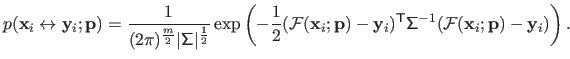 |
(3.18) |
If we apply the principle of MLE of equation (3.11) to equation (3.18), then we obtain the following minimization problem:
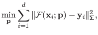 |
(3.19) |
where
 is the Mahalanobis norm.
Equation (3.19) is the very definition of a weighted least-squares minimization problem.
Note that if we further assume that the components of the error vectors
is the Mahalanobis norm.
Equation (3.19) is the very definition of a weighted least-squares minimization problem.
Note that if we further assume that the components of the error vectors
 are i.i.d. or, equivalently, that
, then problem (3.19) reduces to a simple least-squares minimization problem.
The tools that allows one to solve these types of problem have been presented in section 2.2.2.
are i.i.d. or, equivalently, that
, then problem (3.19) reduces to a simple least-squares minimization problem.
The tools that allows one to solve these types of problem have been presented in section 2.2.2.
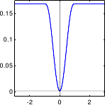
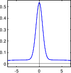
Heavy-tailed Distributions and M-estimators
The data used to estimate the parameters of a model are generally contaminated with noise.
It is a common practice to assume that this noise is normally-distributed.
A common justification for such an assumption is the central limit theorem which states that the sum of a sufficiently large amount of independent random variables is normally-distributed (even if each one of these random variables is not normally-distributed and as long as their mean and variance are defined and finite).
However, it is not always reasonable to assume that the data measurements are normally-distributed.
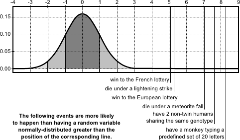
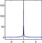
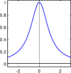
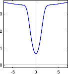
In particular, there can be gross errors in the data, which are extremely unlikely if we only consider a normally-distributed noise (see figure 3.2).
These `false' measurements are called outliers.
Stated otherwise, outliers are arbitrarily large errors.
By contrast, measurements that are not outliers are called inliers.
An estimator is said to be robust when these outliers does not affect much the estimation.
M-estimators are robust estimators that are constructed from MLE (or MAP) assuming a non-normally-distributed noise.
The principle consists in taking a distribution that has a PDF with `heavy tails'.
Having such tails means that large errors are less improbable than it would be with the normal distribution.
Many different M-estimators based upon several noise distributions have been proposed.
Note that some of these M-estimators are statistically grounded in the sense that the considered distributions are related to actual facts.
Other M-estimators are a little bit more artificial in the sense that their underlying probability distributions have been made up for the need of robustness.
Sometimes, the underlying probability distribution of an M-estimator is not even an actual probability distribution since it does not sums up to 1.
In this case, the `probability distribution' is to be considered as some kind of `score function' which takes high values for probable inputs and lower values for less probable inputs.
This does not forbid one to apply the MLE principle to build a cost function.
We now give some notation and vocabulary on M-estimators.
After that, we will detail some typical M-estimators.
An M-estimator is typically defined using what is called a  -function.
The function of an M-estimator is a function from
to
that defines the underlying probability distribution3.2 of the M-estimator:
-function.
The function of an M-estimator is a function from
to
that defines the underlying probability distribution3.2 of the M-estimator:
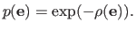 |
(3.20) |
The cost function minimized by the M-estimator is obtained by applying the MLE principle to the distribution of equation (3.20), which gives:
 |
(3.21) |
Note that the least-squares cost function is just a particular case of M-estimator with
 .
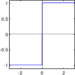
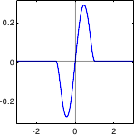
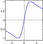
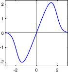
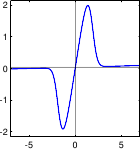
Two other interesting functions can be associated to an M-estimator: the influence function and the weight function.
The influence function, denoted
.
Two other interesting functions can be associated to an M-estimator: the influence function and the weight function.
The influence function, denoted  , is defined as:
 |
(3.22) |
The weight function  , also known as the attenuation function, is defined as:
 |
(3.23) |
It measures the weight given to a particular measurement in the cost function according to the error it produces.
With M-estimators, the principle is to give large weights to small errors and small weights to large errors (which are likely to come from outliers).
Note that, as defined in equation (3.23), the weight function is not defined at zero. It is generally possible to define it at this particular point with a continuous extension.
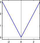
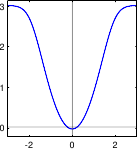
Here comes a list of some typical M-estimators along with some comments.
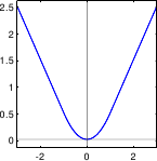
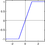
A graphical illustration of these M-estimators is given in figure 3.3.
Other M-estimators can be found in, for instance, (94) or (201).
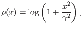
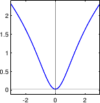
- Least-squares. As it was already mentioned before, the least-squares cost function is a special case of M-estimator with the following -function:
Of course, since it relies on a normally-distributed noise, this `M-estimator' is not robust. In fact, its breakdown point3.3 is 0.
- Least absolute values (
 norm). Instead of using a cost function defined as a sum of square, the least absolute values estimator uses a cost function defined as a sum of absolute values. It corresponds to the following -function:
Although more robust than the least-squares cost function, the norm is not really robust. The main advantage of the norm is that it is convex (which is a nice property for minimizing it). However, problems may arise with the norm since it is not differentiable at 0.
- Huber M-estimator. The Huber M-estimator is a combination of the least-squares cost function and of the norm (100). It is defined with:
with
 a constant that tunes the sensitivity to outliers.
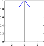
- Tukey M-estimator. The -function of the Tukey M-estimator is the bisquare function:
with
 a constant that tunes the sensitivity to outliers. The Tukey M-estimator is a saturated M-estimator. It means that it takes a constant value after a certain threshold. Some of our contributions will make use of this property. This is one of the most robust M-estimator presented in this document (since the influence of outliers is extremely limited).
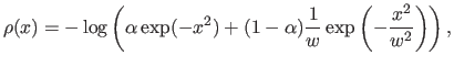
- Cauchy M-estimator. The Cauchy M-estimator is defined by:
where
 is the scale parameter.
It is derived from the Cauchy distribution whose PDF is a bell-shaped curve as for the normal distribution but with heavier tails. The Cauchy distribution is interesting because some of its properties are directly linked to the notion of outlier. For instance, the mean of the Cauchy distribution does not exists. Intuitively, this stems from the fact that the average of the successive outcomes of a Cauchy-distributed random variable cannot converge since it will always be a value so large that it forbids the convergence (as an outlier would do).
is the scale parameter.
It is derived from the Cauchy distribution whose PDF is a bell-shaped curve as for the normal distribution but with heavier tails. The Cauchy distribution is interesting because some of its properties are directly linked to the notion of outlier. For instance, the mean of the Cauchy distribution does not exists. Intuitively, this stems from the fact that the average of the successive outcomes of a Cauchy-distributed random variable cannot converge since it will always be a value so large that it forbids the convergence (as an outlier would do).
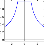
- Modified Blake-Zisserman. The Blake-Zisserman M-estimator (94) relies on the following assumptions: inliers are considered to be normally-distributed while outliers follow a uniform distribution. It is defined with the following -function:
This cost function approximates the least-squares cost function for inliers while it asymptotically tends to
 for outliers. Note that this M-estimator was initially presented in a slightly different way in (23).
- Corrupted Gaussian. The corrupted Gaussian M-estimator assumes a normal distribution for both the inliers and the outliers. However, a Gaussian with a large standard deviation is used for the outliers. It results in the following -function:
here is the ratio of standard deviations of the outliers to the inliers and  is the expected fraction of inliers.
Figure 3.3:
Illustration of the different M-estimators presented in section 3.1.2.2.
|
|
Let
 be the parametric model and let
be the dataset.
Let us denote the -th residual:
be the parametric model and let
be the dataset.
Let us denote the -th residual:
 .
The general form of an M-estimator cost function is:
.
The general form of an M-estimator cost function is:
 |
(3.24) |
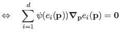
Solving this problem can be achieved with a generic optimization algorithm such as the Newton method.
However, it is possible to turn problem (3.24) into a weighted least-squares problem with variable weights which can be solved with IRLS.
Using IRLS is sometimes preferable than using a generic algorithm such as Newton's method.
Turning problem (3.24) into an IRLS problem is achieved by writing the optimality condition (see section 2.2) and developing them in the following manner:
If we consider the value of
fixed in the factor
 , then equation (3.25) corresponds to the optimality condition of the following weighted least-squares problem:
 |
(3.26) |
with
 .
Therefore, the initial problem (3.24) can be solved with the IRLS principle by iteratively updating the values
.
Therefore, the initial problem (3.24) can be solved with the IRLS principle by iteratively updating the values  for
for
 .
.
Note that minimizing an M-estimator cost function is not a trivial task even though an optimization algorithm is available.
Indeed, the M-estimator cost functions are generally not convex (except for the norm and the Huber M-estimator).
It is thus easy to fall in a local minimum.
Other robust estimators
M-estimators are not the only robust estimators.
There exist other methods that cope with the presence of outliers in the data.
We will not detail here the methods not used in the rest of this document.
For instance, RANSAC (RANdom SAmple Consensus) (70) is a popular robust estimators able to fit a parametric model to noisy data containing outliers.
The least median of squares (64,161) is another robust estimator which consists in replacing the sum of squares in the classical least-squares approach by the median of the squares:
 |
(3.27) |
This approach is based on the fact that the median is a robust statistic while the mean is not (see the next paragraph).
A common technique to solve problem (3.27) is to use a sampling approach.
While this is possible and effective when the number of parameters to estimate is limited, it may become intractable for large numbers of parameters.
Sometimes, it is interesting to get information on the central tendency of a set of values
 .
To do so, using the (arithmetic) mean of the dataset seems to be a natural choice.
However, the mean is not a robust statistic.
Indeed, a single outlier in the dataset can perturb as much as we want this statistic (the breakdown point of the mean is 0).
.
To do so, using the (arithmetic) mean of the dataset seems to be a natural choice.
However, the mean is not a robust statistic.
Indeed, a single outlier in the dataset can perturb as much as we want this statistic (the breakdown point of the mean is 0).
Another measure of central tendency is the median.
The median is the value that separates the higher half and the lower half of the dataset.
Since the outliers are among the highest or the lowest values of the dataset, they do not perturb the median.
The breakdown point of the median is
 .
.
The trimmed mean is another robust central statistic based on the same idea (i.e. that outliers are among the highest or the lowest values of the dataset).
The trimmed is defined as the mean of the central values of the dataset (i.e. the initial dataset with the lowest and highest values removed).
The breakdown point of the trimmed mean is
 , with
  the total number of points.
Contributions to Parametric Image Registration and 3D Surface Reconstruction (Ph.D. dissertation, November 2010) - Florent Brunet
Webpage generated on July 2011
PDF version (11 Mo)