Subsections
Although most of our notation is compliant with the international standard ISO 31-11 (183), we feel that it is appropriate to give the details of the notation most commonly used in this manuscript.
We also give some basic definitions concerning, for instance, some standard operators or matrices.
Scalars are denoted in italic Roman lowercase letters (e.g.  ) or, sometimes, italic Greek lowercase (e.g.
  ).
Vectors are written using bold fonts (e.g.
).
Vectors are written using bold fonts (e.g.
 ).
They are considered as column vectors.
Sans-serif fonts are used for matrices (e.g.
).
They are considered as column vectors.
Sans-serif fonts are used for matrices (e.g.
 ).
The elements of a vector are denoted using the same letter as the vector but in an italic Roman variant.
The same remark holds for matrices.
Full details on notation and tools for vector and matrices will be given in section 2.1.4.
).
The elements of a vector are denoted using the same letter as the vector but in an italic Roman variant.
The same remark holds for matrices.
Full details on notation and tools for vector and matrices will be given in section 2.1.4.
A function is the indication of an input space  , an output space
  , and a mapping between the elements of these spaces.
A function is said to be monovariate when
, and a mapping between the elements of these spaces.
A function is said to be monovariate when
 and multivariate when
 .
All the same way, a function is said to be scalar-valued when
.
All the same way, a function is said to be scalar-valued when  and vector-valued when
 .
We use lowercase italic letters for scalar-valued functions (e.g.
.
We use lowercase italic letters for scalar-valued functions (e.g.  ) and calligraphic fonts for vector-valued functions (e.g.
 ).
From time to time, other typographic conventions are used to denominate functions depending on the context.
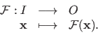
A function
).
From time to time, other typographic conventions are used to denominate functions depending on the context.
A function
 is defined using this notation:
 .
The mapping between an element
.
The mapping between an element
 and its corresponding image
 is denoted
 .
The vector
.
The vector
 is called the free variable (and it can be replaced by any other notation).
The complete definition of a function is written:
is called the free variable (and it can be replaced by any other notation).
The complete definition of a function is written:
 |
(2.1) |
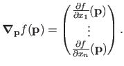
Let
 be a scalar-valued function and let
 be the free variable.
The partial derivative of with respect to
be the free variable.
The partial derivative of with respect to  is denoted by
 .
The gradient of evaluated at
is denoted
.
The gradient of evaluated at
is denoted
 . It is considered as a column vector:
 |
(2.2) |
In practice, the dependency on
is omitted when it is obvious from the context. Consequently,
is often shortened to
 or even
 .
.
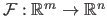
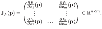
For a vector-valued function
 , the counterpart of the gradient is the Jacobian matrix, denoted
 .
If the components of
are denoted
.
If the components of
are denoted
 then the Jacobian matrix is defined as:
 |
(2.3) |
As for the gradient, the point where the Jacobian matrix is evaluated is omitted when it is clear from the context.
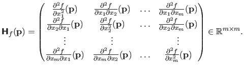
The Hessian matrix of a scalar-valued function
is the matrix of the partial derivatives of second order. This matrix is denoted
 and it is defined by:
 |
(2.4) |
As for the gradient and the Jacobian matrix, we consider that the notation
 is equivalent to the notation
when the vector
is obvious from the context.
is equivalent to the notation
when the vector
is obvious from the context.
The sets are usually written using upper-case letters (e.g.  ).
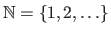
The usual sets of numbers are denoted using the blackboard font:
).
The usual sets of numbers are denoted using the blackboard font:
 for the natural numbers,
 for the integers,
 for the rational numbers,
 for the real numbers, and
 for the complex numbers2.1.
The explicit definition of a set is denoted using the curly brackets (e.g.
for the complex numbers2.1.
The explicit definition of a set is denoted using the curly brackets (e.g.
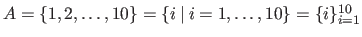 ).
The vertical bar in a set definition is synonym of the expression `such that' (often abbreviated `s.t.').
Following the Anglo-Saxon convention, we consider that
).
The vertical bar in a set definition is synonym of the expression `such that' (often abbreviated `s.t.').
Following the Anglo-Saxon convention, we consider that
 and
and
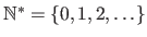 while
is the set of all the real numbers and
while
is the set of all the real numbers and
 .
The set of all the positive (respectively negative) real numbers is denoted
.
The set of all the positive (respectively negative) real numbers is denoted
 (respectively
 ).
The Cartesian product of two sets is designated using the
).
The Cartesian product of two sets is designated using the  symbol, i.e. for two sets
  and
and  , we have
 .
The notation
.
The notation  represents the Cartesian product of with itself iterated
  times.
The symbols used for the intersection, the union, and the difference are respectively
times.
The symbols used for the intersection, the union, and the difference are respectively  ,
,  , and
, and
 .
.
Real intervals are denoted using brackets: ![$ [a,b]$](img63.png) is the set of all the real numbers such that
is the set of all the real numbers such that
 .
The scalars
.
The scalars  and
and  are called the endpoints of the interval.
We use outwards-pointing brackets to indicate the exclusion of an endpoint: for instance,
are called the endpoints of the interval.
We use outwards-pointing brackets to indicate the exclusion of an endpoint: for instance,
![$ ]a,b] = \{ x \in \mathbb{R}\:\vert\:a < x \leq b \}$](img67.png) .
.
Integer intervals (also known as discrete intervals) are denoted using either the double bracket notation or the `three dots' notation.
For instance, the integer interval
 may be written
 or
or
 .
.
Collections, i.e. grouping of heterogeneous or `complicated' elements such as point correspondences are denoted using fraktur fonts (e.g.
 ).
).
Matrices and Vectors
Matrices are denoted using sans serif font (e.g.
).
Although a vector is a special matrix, we use bold symbols for them (e.g.
or
 ).
By default, vectors are considered as column vectors.
The set of all the matrices defined over
and of size
).
By default, vectors are considered as column vectors.
The set of all the matrices defined over
and of size
 is denoted
 .
The transpose, the inverse, and the pseudo-inverse of a matrix
.
The transpose, the inverse, and the pseudo-inverse of a matrix
 are respectively denoted
 ,
,
 , and
, and
 .
The pseudo-inverse is generally defined as
.
The pseudo-inverse is generally defined as
 (see section 2.2.2.6).
The coefficient located at the intersection of the
(see section 2.2.2.6).
The coefficient located at the intersection of the  th row and the
  th column of the matrix
is denoted
th column of the matrix
is denoted  .
The coefficients of a vector are noted using the same letter but with the bold removed.
For instance, the th coefficient of the vector
is written
.
The coefficients of a vector are noted using the same letter but with the bold removed.
For instance, the th coefficient of the vector
is written  .
.
We use either the parenthesis or squared brackets when giving the explicit form of a matrix.
Parenthesis are used when the elements are scalars, e.g. :
 |
(2.5) |
The bracket notation is used when the matrix is defined with `blocks', i.e. juxtaposition of matrices, vectors, and scalars.
For instance:
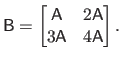 |
(2.6) |
The identity matrix of size
 is denoted
 :
:
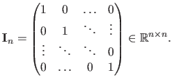 |
(2.7) |
The matrix of size
filled with zeros is denoted
 .
The subscripts in the notation
and
are often omitted when the size can be easily deduced from the context.
.
The subscripts in the notation
and
are often omitted when the size can be easily deduced from the context.
The operator
 is used for the column-wise vectorization of a matrix.
For instance, if
is used for the column-wise vectorization of a matrix.
For instance, if
 :
:
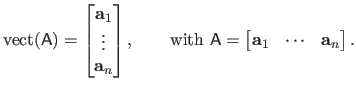 |
(2.8) |
The operator
 deals with diagonal matrices.
The effect of this operator is similar to the one of the diag function in Matlab.
Applied to a vector
deals with diagonal matrices.
The effect of this operator is similar to the one of the diag function in Matlab.
Applied to a vector
 , it builds a matrix
 such that:
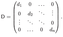 |
(2.9) |
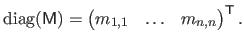
Conversely, when applied to a square matrix
 , the operator
builds a vector that contains the diagonal coefficients of
:
, the operator
builds a vector that contains the diagonal coefficients of
:
 |
(2.10) |
The Hadamard product of two matrices, also known as the element-wise product, is denoted with the  symbol.
The Hadamard product of the matrices
and
symbol.
The Hadamard product of the matrices
and
 is the matrix
 such that
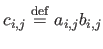 .
The matrices
,
, and
.
The matrices
,
, and
 all have the same size.
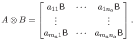
The Kronecker product, denoted with the symbol  , is a binary operation on two matrices of arbitrary sizes.
Let
, is a binary operation on two matrices of arbitrary sizes.
Let
 and
and
 be two matrices.
The Kronecker product of
and
is defined as follows:
be two matrices.
The Kronecker product of
and
is defined as follows:
 |
(2.11) |
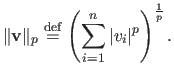
The  -norm of a vector
 is denoted
 .
It is defined for
.
It is defined for  by:
by:
 |
(2.12) |
Note that the 1-norm is also known as the taxicab norm or the Manhattan norm.
The 2-norm corresponds to the Euclidean norm. In this case, we prefer the notation
 instead of the notation
 :
:
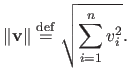 |
(2.13) |
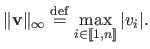
The maximum norm, also known as the infinity norm or uniform norm, is denoted
 . It is defined as:
 |
(2.14) |
Note that the maximum norm corresponds to the -norm when
 .
.
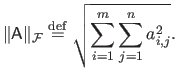
The Frobenius norm of a matrix
is denoted
 . It is defined as:
 |
(2.15) |
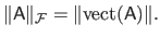
The Frobenius norm of a matrix is related to the Euclidean norm of a vector in the sense that they are both defined as the square root of the sum of the squared coefficients.
In fact, we have the following equality:
 |
(2.16) |
The symbol  means `for all' and the symbol
  means `there exists'.
The symbol
 is synonym of `tends to' (e.g.
 means that tends to the infinite).
Some other notation will surely come during the next few weeks.
Contributions to Parametric Image Registration and 3D Surface Reconstruction (Ph.D. dissertation, November 2010) - Florent Brunet
Webpage generated on July 2011
PDF version (11 Mo)