Subsections
A range surface is a particular type of 3D surface.
It is different from a general 3D surface in the sense that it is defined as a set of depths with respect to 2D coordinates.
A topographic map is a good example of range surface: to each pair (longitude, latitude) is associated an altitude.
In a manner of speaking, range surfaces are a subset of general 3D surfaces.
This is the reason why range surfaces are sometimes called 2.5D surfaces.
An example of range surface is a 3D scene observed from a single point of view.
Compared to a full 3D surface, a range surface may introduce difficulties.
Indeed, even if we consider a continuous 3D world, the range surface corresponding to a point of view may have discontinuities.
Discontinuities are generally hard to handle.
Mathematically speaking, range surfaces are adequately modelled by scalar-valued functions from
 (or a subset of it) to
 .
Such surfaces are also known as Monge patches (86).
Figure 4.1 gives an example of range surface.
.
Such surfaces are also known as Monge patches (86).
Figure 4.1 gives an example of range surface.
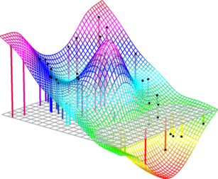
Figure 4.1:
An example of range surface. In a range surface, an elevation is associated to each couple of 2D points on the plane of the grey grid.
|
 |
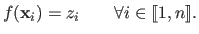
Range data are data points which follow the same principle as range surfaces.
Range data points are written using the following notation:
 |
(4.1) |
where
 is the altitude (or elevation, or depth) corresponding to the 2D point
 .
Note that
.
Note that
![$ \left [ \mathbf{x}^\mathsf{T} z \right ] ^\mathsf{T}$](img793.png) is a classical 3D point.
An example of range data points is given in figure 4.2.
is a classical 3D point.
An example of range data points is given in figure 4.2.
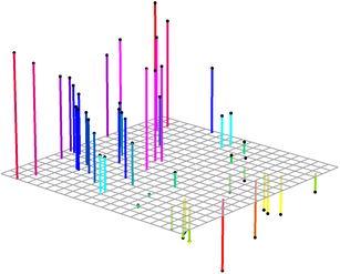
Figure 4.2:
An example of range data points (black dots). The coloured segments represent the depth of each point.
|
 |
A depth map is a set of range data points organized on a regular and uniformly spaced grid4.1.
In other words, a depth map is like a standard digital picture (i.e. an array of numbers each one of which coding for a colour or a level of grey) but the numbers represent distances instead of colours.
The individual elements of a depth map are still named pixels even though they are not `little squares of colours' but elementary pieces of surface.
Nowadays, there exists many approaches and sensors to acquire range data.
We emphasize here that the acquisition of range data is not the central topic of this thesis.
We are more interested in the processing of range data than in its acquisition.
Therefore, we only give a brief overview of the ways in which range data may be acquired.
The devices that allows one to acquire range data may be categorized into two classes:
- Passive sensors.
- The central part of the capturing device is a `simple' passive sensor such as a CMOS or a CCD sensor. Nothing is emitted from the device. The acquisition of range data with such sensors is therefore completely non-intrusive in the sense that the observed scene is not `modified' for the acquisition. The main part of these approaches generally relies on complex algorithms.
- Active sensors.
- In a way or another, the capturing device illuminates the scene in order to get supplementary information about its geometry. The data acquired with such sensors are generally of better quality than with passive sensors. However, these sensors are more invasive4.2 than passive sensors. Complex algorithms are also used in the acquisition process.
We give here a non-exhaustive list of passive technique for acquiring range data.
As we already mentioned, we do not pretend to make a detailed review on range data acquisition.
However, each one of the succinctly described method is associated to some references.
It is a common practice to name these techniques with the prefix `Shape-from-'.
As a casual remark, it would have been more correct to use the prefix `Range-from-'.
Stereo reconstruction is an important problem in computer vision which has been addressed in many ways.
In a certain sense, it consists in emulating the human vision by exploiting the discrepancies between two images of the same scene taken from a different point of view.
The core principle is to use the discrepancies between two images of the same scene to infer 3D information.
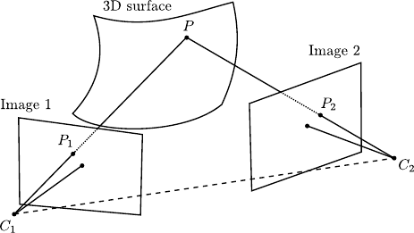
This may be achieved using, for instance, point triangulation and epipolar geometry (see figure 4.3).
The interested reader may found a complete review of such techniques in documents such as (68,94,14,69,196).
Other approaches exist such as the reconstruction of discrepancy maps (105,26,167)
Figure 4.3:
Illustration of the basic principles of shape-from-stereo (stereo reconstruction). The reconstruction of a 3D point may be achieved using the epipolar geometry.
|
 |
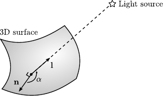
Shape-from-shading is a technique that reconstruct the 3D structure of a scene from the lighting of the object.
Detailed information on shape-from-shading may be found in (199).
Usually, some general assumptions are made.
For instance, one may consider that there is only one light source.
One may further assume that the surfaces of the scene exhibits Lambertian reflectance which means that the intensity reflected by a surface to an observer is the same regardless of the observer's angle of view.
We may then apply the Lambert's cosine law which state that the intensity  of a surface at a given point is given by:
 |
(4.2) |
with
 a vector pointing from the surface to the light source,
 the surface's normal vector,
  the colour of the surface, and
  the intensity of the light source (see figure 4.4).
By definition of the scalar product of two vectors, we then have that
the intensity of the light source (see figure 4.4).
By definition of the scalar product of two vectors, we then have that
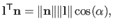 |
(4.3) |
where  is the angle between the vectors
and
.
In shape-from-shading, the observed intensity is used to compute a field of normal vectors of the surface with equation (4.3).
This field is then integrated to reconstruct the surface.
is the angle between the vectors
and
.
In shape-from-shading, the observed intensity is used to compute a field of normal vectors of the surface with equation (4.3).
This field is then integrated to reconstruct the surface.
Figure 4.4:
Illustration of Shape-from-Shading. Under some assumptions about the observed surface and the lighting conditions, it is possible to retrieve a field of normal vectors from the colour of the surface. The actual 3D surface is obtained by integrating the vector field.
|
 |
Shape-from-Motion is a technique that retrieve the shape of a scene from the spatial and temporal changes occurring in an image sequence.
More details on this technique may be found in (60,184,15,138,59).
To some extent, it is similar to shape-from-stereo.
There are nonetheless some important differences.
In particular, the typical discrepancies between two successive images are much smaller than those of typical stereo pairs.
This makes shape-from-motion more sensible to noise than shape-from-stereo.
Another important difference is the fact that the transformation linking two consecutive frames is not necessarily a single rigid 3D transformation.
Compared to shape-from-motion, shape-from-motion has its advantages.
For instance, pixel correspondences may be easier to find with shape-from-motion since the baseline is smaller than with typical shape-from-stereo.
Shape-from-focus is a technique that reconstruct range data by acquiring two or more images of the same scene under various focus settings (133).
Once the best focused image is found, a model that links focus and distance is used to determine the distance.
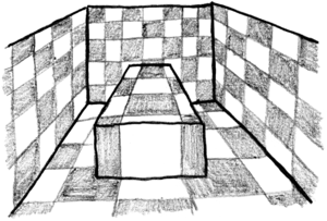
Shape-from-texture is a technique that relies on the deformation of the individual texels (texture elements) to retrieve 3D information from a scene.
Complementary information on this technique may be found in (4).
The shape reconstruction typically exploits two types of distortion: perspective and foreshortening transformations (see figure 4.5).
The perspective distortion makes the objects far from the camera appear smaller.
The foreshortening distortion makes objects not parallel to the image plane shorter.
It is possible to estimate the amount of those distortions from the textures contained in an image.
As for other methods described in this section, the raw output of this algorithm is a discrete field of normal vector to the observed surface.
If this field is dense enough and if the assumption of a smooth surface is made, then it is possible to recover the whole surface shape.
Figure 4.5:
Illustration of Shape-from-Texture. This technique exploits the local transformations (perspective and foreshortening deformations) of the texture to reconstruct a field of normal vectors to the surface.
|
 |
We now explain the basic principles of a few active sensors used to acquire range data.
We only consider sensors commonly used in computer vision.
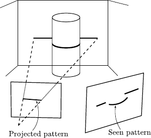
Structured light is a technique to reconstruct the geometry of the scene that uses a light projector and an intensity camera placed at a distance from each other.
Detailed information on this technique may be found in (200).
The projector emits a light pattern (whose shape is perfectly known).
For instance, the pattern may be a simple line.
From the point of view of the camera, the projected line is a distorted curve whose shape depends on the shape of the scene.
Figure 4.6:
Basic principles of 3D reconstruction using structured light: a pattern with known shape is projected on the scene. A camera observes the pattern. An algorithm deduces the shape of the scene from the deformation of the pattern.
|
 |
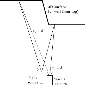
LIDAR (LIght Detection And Ranging) is an optical sensor that measures properties of reflected light to determine the distance of a distant target.
The LIDAR technology is also known under the acronym LADAR (LAser Detection And Ranging).
In a nutshell, it relies on the same principles as the standard RADAR.
The main difference is that RADAR uses radio waves while LIDAR uses much shorter wavelength (typically in the ultraviolet, visible, or near infrared range).
Given the fact that such sensors are generally not able to detect objects smaller than the wavelength they use, LIDAR is able has a much finer resolution than RADAR.
The distance of an object is determined by measuring the time delay between the transmission of a pulse and detection of the reflected signal (see figure 4.7).
A laser has a very narrow beam.
This allows one to make a measurements at a very fine precision.
Note that the measurements are generally `point-wise', i.e. the distance of only one point is computed.
Having a complete range map of a scene requires one to make multiple measurements.
Since there is necessarily a delay between two measurements, it can be a problem if the scene is not strictly rigid.
Figure 4.7:
Basic principle of LADAR. With this technique, point-wise measurements of depths are achieved by measuring the time delay between the emission of a laser pulse and the reception of that pulse by a special sensor.
|
 |
The general principle of time-of-flight (ToF) cameras is similar to that of LIDAR sensors.
However ToF cameras have the advantage of being able to capture a whole scene at the same time.
Besides, ToF cameras can provide up to 100 images (range maps) per second.
Additional informations on ToF cameras may be found in (65,82,191,116,197).
ToF cameras have been used in many fields such as medical imaging (140,189), augmented reality (10,107), intelligent vehicles (99).
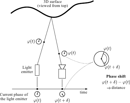
The general principle of ToF cameras is illustrated in figure 4.8.
The device is made of two parts: a near infrared light source and an optical sensor.
The light source emits a phase-modulated signal.
The optical sensor is a `variant' of a standard CMOS sensor: in addition to the intensity of the reflected light, it is also able to capture the phase of the received signal.
The signal modulation is synchronized between the light source and the optical sensor.
For each pixel of the optical sensor, the depth is computed by comparing the current phase modulation (at the time of reception) with the phase of the received signal.
Note that there exist ToF cameras that use slightly different principle for retrieving depths.
However, the principle described above is the one used by the cameras we had access to, namely the products from PMDTec4.3 (cameras 19k-S) and Mesa Imaging4.4 (SwissRanger 3000 and SwissRanger 4000).
Figure 4.8:
Basic principle of ToF cameras. ToF cameras are able to capture range maps by measuring a phase delay for each one of the pixels.
|
 |
Although very useful and efficient, ToF cameras have also some drawbacks.
For instance, they have a resolution which is quite limited if we compare them to the typical resolutions of standard digital cameras.
The range of non-ambiguous distances is also limited: typically 7 metres.
This range may be increased but it is achieved to the detriment of the depth precision.
Another drawback of ToF cameras is that the depth measurements are influenced by the material (mainly by its reflexivity).
The accuracy of the measurements are also influenced by multiple reflexions of the emitted infrared signal (this phenomenon often happens when the observed scene has concave corners).
The measurements may also be perturbed by ambient light.
As a consequence of these drawbacks, the depth maps acquired with ToF cameras are usually extremely noisy.
However, one should put these disadvantages into perspective since ToF cameras are amongst the only sensors able to provide 3D information in real-time (and with a high acquisition rate) regardless of the appearance of the observed scene4.5.
An Introductory Example
In this section, we present an example that illustrates the basic principle for fitting a parametric surface to range data.
More generally, this example is also the occasion to make concrete the theoretical tools presented in the previous chapters.
In particular, we will show how parametric estimation can be achieved with range data.
We also give an example of automatic hyperparameter selection.
More advanced topics on range surface fitting, including our contributions, will come later in this chapter.
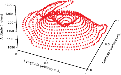
In this example, we use geographical range data extracted from a topographic map4.6.
The data, shown in figure 4.9, represent Puy Pariou, an extinct volcano near Clermont-Ferrand.
Here, the data does not have any particular structure.
In particular, the data points are not arranged on a regular grid.
As they were extracted manually from a topographic map, there is not much noise in the data points.
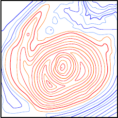
Figure 4.9:
Example of range data representing the Puy Pariou, a volcano in Chaîne des Puys next to Clermont-Ferrand, France. (a) Data represented as points. (b) Data represented with contour lines.
|
 |
 |
| (a) |
(b) |
|
We now give an (oversimplified) approach to range surface fitting.
Given a set of range data points
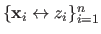 , the goal of range surface fitting is to find a function
 that fits the data point, i.e.:
 |
(4.4) |
In practice, the equality in equation (4.4) does not make much sense.
Indeed, there is usually noise in the data points.
This noise can come from the underlying physics of the sensor used to acquire the data (such as a Time-of-Flight camera or a LIDAR).
Let us note
 the true surface.
The available data may be seen as a noisy discretization of the true surface, i.e.:
the true surface.
The available data may be seen as a noisy discretization of the true surface, i.e.:
 |
(4.5) |
where the
 (for
(for
 ) are random variables.
The goal of range surface fitting is to find a function
) are random variables.
The goal of range surface fitting is to find a function  as close as possible of
.
as close as possible of
.
This problem can be turned into a parameter estimation problem.
It means that the range surface fitting problem will be formulated as a minimization problem, that consists in finding a set of parameters
 that minimizes a certain cost function.
From this point of view, one must answer the following five questions:
that minimizes a certain cost function.
From this point of view, one must answer the following five questions:
- What parametric model should we use?
- What is the probability distribution of the noise (given equation (4.5), we have already assume that the noise is additive)?
- What assumptions (priors) can we make about the surface to reconstruct?
- What optimization algorithm can be used?
- How can the hyperparameters be automatically selected?
In the next paragraphs, we discuss these five points and illustrate them using our example of range surface fitting with simplified assumptions.
Note that this set of five questions is quite generic in the sense that they have to be answered for almost any parametric estimation problem.
The choice of a correct parametric model is important.
It must be flexible enough to be able to model correctly the data.
Ideally, the true surface
should be a special case of the parametric model.
In other words, if
 is the parametric function model, there should exist a set of parameters
 such that
 .
In practice, such a condition is difficult to satisfy because
is unknown and it may vary in great proportion.
Therefore, the function model is just expected to have enough degrees of freedom.
One should also take care of the fact that the parametric model should be simple enough in order to get tractable computations.
.
In practice, such a condition is difficult to satisfy because
is unknown and it may vary in great proportion.
Therefore, the function model is just expected to have enough degrees of freedom.
One should also take care of the fact that the parametric model should be simple enough in order to get tractable computations.
For the range surface fitting problem, we may use a uniform cubic B-spline model with a relatively high number of control points.
This choice is motivated by the fact that such a model is quite generic, has a high number of degree of freedom, and generally leads to `simple' computations.
Determining the `nature' of the noise allows one to derive a proper cost function using, for instance, one of the statistical approaches presented in section 3.1.1, namely Maximum Likelihood Estimation (MLE) or Maximum A Posteriori Estimation (MAP).
A good model of the noise is particularly important to cope with noise and outliers.
In our specific example, we consider that the errors
(for
) are all normally-distributed with zero mean and that they all have the same variance.
We also assume that the errors are independent.
Such an hypothesis on the noise is generally a reasonable choice.
Besides, it naturally leads to a least-squares optimization problem, as explained in section 3.1.2.1.
A proper parametric model and a proper model of noise may not be sufficient to fit a surface to range data.
For example, if the number of degrees of freedom of the parametric model is greater than the number of data points, it will result in an under-constrained problem.
Even if there are enough data points, there still can be ambiguities due to the noise: is a small bump in the data just a noisy measurement or the true shape of the surface?
These problems can be addressed by using a MAP estimation scheme with extra assumptions on the surface.
For instance, one may require the surface to be `smooth'.
In our example, we want the surface to minimize the bending energy (while still being close to the data points, of course).
The bending energy is defined by:
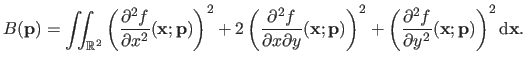 |
(4.6) |
More will come about the bending energy in the sequel of this document.
For now, let us just say that the lower the bending energy the smoother the surface and that a surface of minimal bending energy is a plane.
Imposing a small bending energy can be seen as a physical prior on the surface.
Indeed, it is equivalent to say that a set of parameters leading to a smooth surface is more probable than another set of parameters.
This can be formulated in statistical terms by saying that, for instance, we have a prior probability defined as:
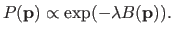 |
(4.7) |
Such an expression makes surfaces with minimal bending energy the most probable surfaces and this probability decreases when the bending energy becomes higher.
The parameter  controls the width of the bell-shaped curve defined by equation (4.7).
A small results in a wide bell-shaped curve which means that surfaces with high bending energy are possible with a reasonably high probability.
On the contrary, a high value for results in a narrow bell-shaped curve which is equivalent to say that surface with high bending energy are utmost improbable.
controls the width of the bell-shaped curve defined by equation (4.7).
A small results in a wide bell-shaped curve which means that surfaces with high bending energy are possible with a reasonably high probability.
On the contrary, a high value for results in a narrow bell-shaped curve which is equivalent to say that surface with high bending energy are utmost improbable.
The assumptions made on the noise and on the surface prior together with the MAP principle leads to the following minimization problem:
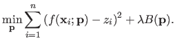 |
(4.8) |
Since we decided to use the B-spline model and given the expression of the bending energy  , the cost function in equation (4.8) is a sum of squared terms, each one of which being linear with respect to the parameters
 .
Consequently, equation (4.8) is a linear least squares minimization problem.
The tools and algorithms described in section 2.2.2.6, section 2.2.2.8, section 2.2.2.9, and section 2.2.2.10 can thus be used to solve this minimization problem.
.
Consequently, equation (4.8) is a linear least squares minimization problem.
The tools and algorithms described in section 2.2.2.6, section 2.2.2.8, section 2.2.2.9, and section 2.2.2.10 can thus be used to solve this minimization problem.
In this example, we consider that the only hyperparameter of interest is the regularisation parameter in problem (4.8).
It is reasonable to make this assumption.
Indeed, one could also have considered the number of control points of the B-spline.
We think that, in this context, it is simpler to consider a large number of control points.
The resulting high complexity of the model is then compensated by the regularisation prior.
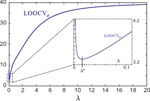
In this example, we have decided to use the ordinary cross-validation approach to automatically determine a proper value for the regularization parameter.
Since problem (4.8) is a linear least-squares optimization problem, it is possible to use the closed-form formula for computing this criterion.
The profile of the cross-validation criterion is give in figure 4.10.
The final result of the range surface fitting process is shown in figure 4.11 (b).
Figures 4.11 (a) and (c) respectively illustrate the overfitting and underfitting phenomena that arise if the regularization parameter is not properly chosen.
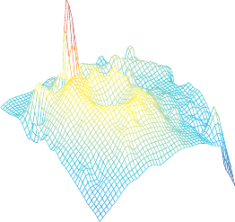
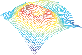
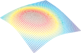
Figure 4.11:
Final results for our example of range surface fitting. (a) Overfitting phenomenon (the prior on the regularisation is not strong enough and, consequently, the complexity of the surface model is much larger than the actual complexity of the data). (b) Correct regularization parameter chosen by minimizing the cross-validation criterion. (c) Underfitting phenomenon (the large regularization parameter overly reduces the effective complexity of the model).
|
|
Contributions to Parametric Image Registration and 3D Surface Reconstruction (Ph.D. dissertation, November 2010) - Florent Brunet
Webpage generated on July 2011
PDF version (11 Mo)