Subsections
The L-Tangent Norm
In this section, we expose one of our contributions concerning range surface fitting.
This work was first published in (31).
As it was previously presented, range surface fitting is commonly achieved by minimizing a compound cost function that includes two terms: a goodness of fit term and a regularization term.
The trade-off between these two terms is controlled by the so-called regularization parameter.
Many approaches can be used to determine automatically a proper value for this hyperparameters.
Some, such as the cross-validation, are very generic.
We already reviewed them in section 3.2.2.
Some others are more specific in the sense that they have been designed to work with the type of cost function considered in this section, i.e. a mix of a data term and a regularization term.
This is the case of the L-curve approach (which will be detailed later in this section).
However, all these methods are not fully satisfactory.
Indeed, the methods based on cross-validation generally suffer from their computational complexity.
The L-curve is more efficient in terms of the computational burden but the resulting criterion is hard to minimize in the sense that there are usually many local minima.
Therefore, we propose a new criterion to tune the regularization parameter in the context of range surface fitting.
We called this new criterion the L-Tangent Norm (LTN).
Even though empirical, the LTN gives sensible results with a much lower computational cost.
This section is organized as follows.
Firstly, we give supplemental details on range surface fitting.
In particular, we give the details on the bending energy term for the B-spline model.
Secondly, we review another criterion for hyperparameter selection: the L-curve criterion.
Thirdly, we present our new criterion: the L-Tangent Norm.
Finally, we conclude with some experimental results on both synthetic and real data.
The main building blocks of range surface fitting have been presented in the introductory example of section 4.1.3.
In this section, we also use the B-spline model to represent the surface.
We use the same principle as the one utilized in the introductory example.
However, we use a slightly different way of writing it:
 |
(4.9) |
where
 is the data term that measures the discrepancy between the fitted surface and the data, and
 is the bending energy term that measures how `smooth' the surface is.
Besides, the regularization parameter is reparametrized so that it lies within
is the bending energy term that measures how `smooth' the surface is.
Besides, the regularization parameter is reparametrized so that it lies within  instead of
 .
If we denote by
.
If we denote by
 the parametric model of surface, then we have that:
where
 is the definition domain of the range surface.
It can be chosen as, for instance, the bounding box of the data points.
Since
is the definition domain of the range surface.
It can be chosen as, for instance, the bounding box of the data points.
Since  is a tensor-product B-spline, it can be written as a linear combination of the control points, i.e. :
 |
(4.12) |
where
 is the vector defined by (with
 ):
):
 |
(4.13) |
Consequently the data term
can be written in matrix form:
 |
(4.14) |
where
 is the matrix such that
 and
and
 is obtained by stacking the depth of the data points, i.e.
 .
The bending term can also be written as the squared norm of some vector.
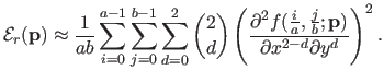
One trivial way of doing it would be to approximate the bending energy term of equation (4.11) by discretizing the integral over a regular grid:
.
The bending term can also be written as the squared norm of some vector.
One trivial way of doing it would be to approximate the bending energy term of equation (4.11) by discretizing the integral over a regular grid:
 |
(4.15) |
Since the second derivatives of a B-spline are also linear with respect to the control points, the approximation of equation (4.15) is a sum of squared terms linear with respect to the parameters.
Even though this approach is effective in practice, there is a better way to write the bending energy term as a squared norm of a vector.
Indeed, we showed that it was possible to get an exact formula for the bending energy of the form:
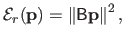 |
(4.16) |
where
 is a matrix that we call the bending matrix.
The details of the computations of the bending matrix will be given in section 4.2.1.2.
For now, let us just assume that the matrix
is a matrix that we call the bending matrix.
The details of the computations of the bending matrix will be given in section 4.2.1.2.
For now, let us just assume that the matrix
 exists.
Given all the previous elements, the initial minimization problem of equation (4.9) is equivalent to the following linear least-squares minimization problem in matrix form:
exists.
Given all the previous elements, the initial minimization problem of equation (4.9) is equivalent to the following linear least-squares minimization problem in matrix form:
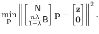 |
(4.17) |
The solution to this problem is given by using, for instance, the normal equations.
For a given regularization parameter
 , we get that:
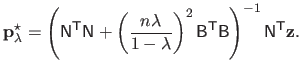 |
(4.18) |
The Bending Matrix
In this section, we show how the bending matrix
can be derived and practically computed.
To the best of our knowledge, the practical computation of the bending matrix cannot be found in the literature.
For the sake of simplicity, we first consider the case of a univariate and scalar-valued B-spline.
For the same reasons, we also restrict this section to uniform cubic B-splines, which is the flavour of B-spline the most used in this thesis.
Let be the B-spline with knot sequence
 .
We consider the bending energy over the natural definition domain of the B-spline, i.e. :
.
We consider the bending energy over the natural definition domain of the B-spline, i.e. :
 |
(4.19) |
The integral bending energy can be divided on each knot interval and, therefore, equation (4.19) can be rewritten as:
 |
(4.20) |
As we have seen in section 2.3.2.3, the B-spline may written as:
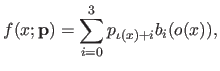 |
(4.21) |
where the four functions  (for
(for
 ) are the pieces of the B-spline basis functions.
The functions
) are the pieces of the B-spline basis functions.
The functions  and
and  were defined in section 2.3.2.3.
A similar notation is possible for the derivatives of the B-spline:
were defined in section 2.3.2.3.
A similar notation is possible for the derivatives of the B-spline:
 |
(4.22) |
where  is the width of a knot interval (i.e.
 for all
 ).
The function
).
The function  is the derivative of the
  -th order of the function (for
).
In particular, for the second derivatives (
-th order of the function (for
).
In particular, for the second derivatives ( ), we have that:
 |
 |
(4.23) |
 |
 |
(4.24) |
 |
 |
(4.25) |
 |
 |
(4.26) |
Here is a formula which will be useful for the computation of the bending matrix: the integration by substitution.
It is given by:
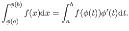 |
(4.27) |
We now compute
 i.e. the bending energy of a B-spline over the knot interval
![$ [k_j,k_{j+1}]$](img857.png) .
.
 |
 |
(4.28) |
| |
 |
(4.29) |
| |
 |
(4.30) |
| |
 |
(4.31) |
| |
 |
(4.32) |
| |
 |
(4.33) |
| |
 |
(4.34) |
| |
 |
(4.35) |
| |
 |
(4.36) |
| |
 |
(4.37) |
| |
 |
(4.38) |
| |
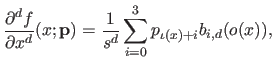
![$\displaystyle = \frac{1}{s^3} \bar{\mathbf{p}}^\mathsf T \mathsf{M}_2^\mathsf T...
...& x^2/6 x^2/6 & x/9 \end{pmatrix}} \right]_0^1 \mathsf{M}_2 \bar{\mathbf{p}}$](img870.png) |
(4.39) |
| |
 |
(4.40) |
| |
 |
(4.41) |
| |
 |
(4.42) |
| |
 |
(4.43) |
where
 is the matrix defined as:
 |
(4.44) |
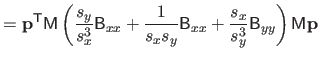
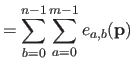
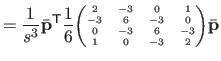
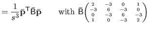
The bending matrix for the bending energy over the entire natural definition domain is obtained by summing the bending matrix for single knot intervals.
Therefore, if we define the bending matrix as:
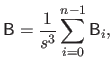 |
(4.45) |
then the bending energy is given by:
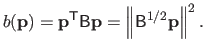 |
(4.46) |
Note that in practice, one generally does not need to explicitly compute a square root of the matrix
.
This stems from the fact that it is usually the form
 which is used in practical computations.
The bending matrix is interesting for several reasons.
Of course, it is nice to have an exact formula of the bending energy that can easily be integrated into a linear least-squares optimization problem.
Besides, the bending matrix as defined in equation (4.45) is a sparse matrix.
Indeed,
is an heptadiagonal symmetric matrix.
This sparsity structure allows one to use efficient optimization algorithms.
The last interesting property of this bending matrix is that it is usually much smaller that the matrix that would arise by using the approximation of equation (4.15).
Indeed,
is a matrix of
 .
With the approximate formula, the resulting matrix has usually much more rows (it depends on the fineness of the grid used for the discretization of the integral).
.
With the approximate formula, the resulting matrix has usually much more rows (it depends on the fineness of the grid used for the discretization of the integral).
We now derive an exact formula for the bending energy term for bivariate spline.
This derivation follows the same principle as the one used for the univariate case.
Let be the uniform cubic tensor-product bi-variate B-spline with knots
 along the
  direction and
 along the
  direction.
The bending energy, denoted
direction.
The bending energy, denoted  , is defined by:
 |
(4.47) |
As in the univariate case, the bending energy term over the entire natural definition domain can be split on each knot domain:
 |
(4.48) |
where
 is the bending energy of the B-spline over the knot domain
![$ [k_a^x,k_{a+1}^x] \times [k_b^y,k_{b+1}^y]$](img887.png) .
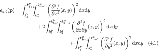
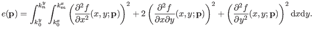
The bending energy
can be further split in three terms:
.
The bending energy
can be further split in three terms:
We will give the details of the computation only for the first term in equation (4.49) since the two other terms are computed in an almost identical way.
But before that, we define a few other notation.
As it was explained in section 2.3.2.5, the bivariate B-spline can be written as:
 |
(4.49) |
where
 ,
,
 is the geometric matrix (defined in equation (2.99)), and
 is the vector of
 defined as a function of the free variable by:
 |
(4.50) |
The partial derivatives of the bi-variate spline can be written in a similar way:
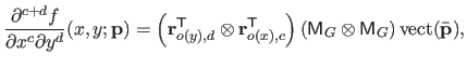 |
(4.51) |
where
 is the derivative of the
  th order of the vector
  .
Along the direction, these vectors are given by:
.
Along the direction, these vectors are given by:
 |
 |
(4.52) |
 |
 |
(4.53) |
 |
 |
(4.54) |
 |
 |
(4.55) |
where  is the width of a knot interval along the direction (i.e.
 for all
 ).
These formulas are identical for the direction expect for which is replaced by
).
These formulas are identical for the direction expect for which is replaced by  , the width of a knot interval along the direction.
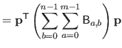
The second and the third terms of
are computed in a similar way as the first term.
We obtain the following formulae:
Consequently, the exact formula for the bending energy over the knot domain
is:
Finally, the bending energy for the entire natural definition domain is:
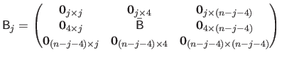
In the bivariate case, the bending matrix
has similar properties than the bending matrix in the univariate case.
In particular, the matrix
is still sparse ;
although its sparsity pattern is a bit more complicated.
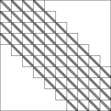
Indeed, it is made of 7 diagonals of blocks each one of which being an heptadiagonal matrix.
This is illustrated in figure 4.12.
Figure 4.12:
Sparsity structure of the bending matrix of bi-variate B-splines. Note that all the blocks are heptadiagonal matrices but they are not all identical to each others. The entire bending matrix is symmetric as are the individual heptadiagonal blocks.
|
 |
The L-Curve Criterion
The L-curve criterion is a criterion used to automatically determine a regularization parameter in an inverse problem.
It was first introduced in (109).
This criterion is not as generic as the criteria reviewed in section 3.2.2.
Indeed, it is specifically designed to determine only one type of hyperparameter (a regularization parameter) in the special context of a least-squares cost function.
The interested reader may find an extensive review of the L-curve criterion in, for instance, (93,124,92,157).
The underlying idea of the L-curve criterion is to find a compromise between underfitting and overfitting.
We remind the reader that
 is the vector of the control points solution to the problem (4.17) for a given regularization parameter
  .
Let
.
Let
 be the residual norm and let
 be the solution norm4.7.
In an underfitting situation, the solution norm is expected to be small while the residual norm is likely to be large.
On the contrary, in an overfitting situation, the solution norm is probably large and the residual norm is expected to be small.
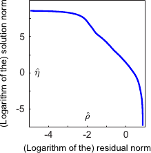
To find a compromise between these two pathological situation, the principle of the L-curve criterion is to plot the residual norm and the solution against each other.
More precisely, it is the logarithm of the residual norm and of the solution norm that are plotted against each others.
This allows one to be invariant to the scale.
The resulting curve is called the L-curve.
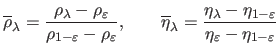
If we note
be the solution norm4.7.
In an underfitting situation, the solution norm is expected to be small while the residual norm is likely to be large.
On the contrary, in an overfitting situation, the solution norm is probably large and the residual norm is expected to be small.
To find a compromise between these two pathological situation, the principle of the L-curve criterion is to plot the residual norm and the solution against each other.
More precisely, it is the logarithm of the residual norm and of the solution norm that are plotted against each others.
This allows one to be invariant to the scale.
The resulting curve is called the L-curve.
If we note
 and
and
 the two functions such that
 and
and
 , then the L-curve is the set:
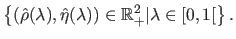 |
(4.63) |
The name L-curve comes from the usual shape of this curve.
Indeed, it often resembles to the letter L.
The extremities of the L correspond to the underfitting and overfitting situations.
The compromise selected with the L-curve criterion corresponds to the corner of the L.
This corner has often been selected manually by actually plotting the L-curve.
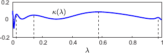
It is possible to make this approach automatic by saying that the corner of the L is the point of the curve which as the highest curvature.
Let  be the curvature of the L-curve:
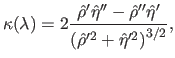 |
(4.64) |
where the symbols  and
and  denote respectively the first and the second derivatives of the functions to which it is applied.
The L-curve criterion is thus defined as:
denote respectively the first and the second derivatives of the functions to which it is applied.
The L-curve criterion is thus defined as:
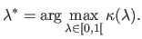 |
(4.65) |
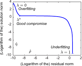
An example of L-curve is shown in figure 4.13.
Figure 4.13 also shows the typical aspect of the L-curve criterion. In this example, the L-curve has actually the shape of the letter L.
In this case, the L-curve criterion is well defined in the sense that its maximum indeed corresponds to a good regularization parameter.
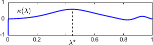
Figure 4.13:
(a) An example of L-curve that has the typical shape of the letter L. The extremities of the L corresponds to the worst cases: underfitting and overfitting. (b) Curvature of the L-curve shown in (a). The highest curvature corresponds to the regularization parameter determined with the L-curve criterion.
|
 |
 |
| (a) |
(b) |
|
However, selecting a regularization parameter with the L-curve criterion is not always that simple.
Indeed, the L-curve is often not well defined in the sense that there are a lot of local maxima.
This is a problem if we want a fully automatic approach to choose the regularization parameter.
Besides, when the values of the maxima are close to each other, it is not always clear to decide which local maxima is the best (it is not necessarily the highest one: it can be one of the highest).
This pathological situation is illustrated in figure 4.14.
Figure 4.14:
An example of pathological case for the L-curve criterion.
|
 |
 |
| (a) |
(b) |
|
The L-Tangent Norm (LTN) is a new criterion that we have designed to choose the regularization parameter in range surface fitting.
It was partly inspired by the idea of `stability' developed in (151).
It also relies on the L-curve.
One thing that can easily be noticed when dealing with L-curves is that their parametrization is not uniform. In particular, one can observe that there exists a range of values for where the tangent vector norm is significantly smaller than elsewhere.
Our new criterion is based on this observation. The regularization parameter is chosen as the one for which the L-curve tangent norm is minimal. Intuitively, such a regularization parameter is the one for which a small variation of the regularization parameter has the lowest impact in the trade-off between the goodness of fit and the surface smoothness.
The L-Tangent Norm (LTN) criterion can be written as:
 and
and
 are the derivatives with respect to of the normalized residual and solution norms:
 |
(4.68) |
for
 a small positive constant (
 , for instance).
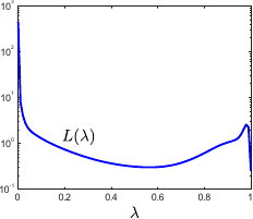
A typical example of the L-tangent norm criterion is shown in figure 4.15.
Even if our criterion is not convex, it is continuous and smooth enough to make it interesting from the optimization point of view.
Moreover, neglecting the values of very close to 1, our criterion often has a unique minimum, which is not the case of the L-curve criterion.
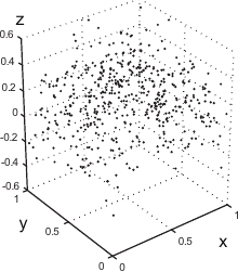
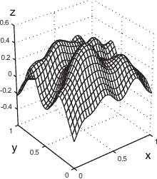
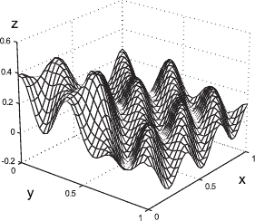
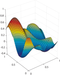
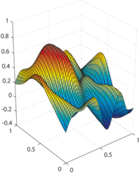
Figure 4.15:
Example of the L-Tangent Norm criterion. (a) An initial surface. (b) The initial surface sampled on a set of 500 points with additive normally-distributed noise. (c) The L-Tangent Norm criterion. (d) The reconstructed surface using the optimal regularization parameter found with the LTN.
|
|
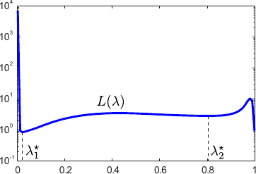
It sometimes happens that there are two minima.
In such cases, it seems that these two local minima are both meaningful.
The smaller one (i.e. the global minimum) corresponds to the regularization parameter giving the best of the two `explanations' of the data.
The second one seems to appear when the data contains, for instance, a lot of small oscillations.
In this case, it is not clear (even for a human being) whether the surface must interpolate the data or approximate them, considering the oscillations as some kind of noise.
This situation is illustrated in figure 4.16.
The evaluation of the LTN criterion requires only the computation of the residual and solution norm derivatives.
This makes our new criterion faster to compute than, for instance, cross-validation.
In particular, our criterion allows one to improve the computation time when the surface model leads to sparse collocation and regularization matrices (as it is the case with the B-spline model).
This is not possible with the cross-validation because the influence matrix is generally not sparse.
Another advantage of the LTN criterion is that it would still be efficient with a non-linear surface model.
While cross-validation needs a non-iterative formula to achieve acceptable computational time (which does not necessarily exists for such surface models), our criterion just needs the computation of the residual and the solution norms.
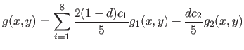
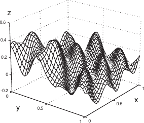
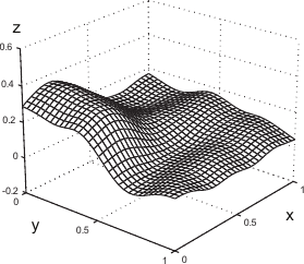
The first type of data we have used in these experiments are generated by taking sample points (with added noise) of surfaces defined by:
where
 are randomly chosen in
 ![$ [0,1]$](img649.png) and where is randomly chosen in
and where is randomly chosen in  .
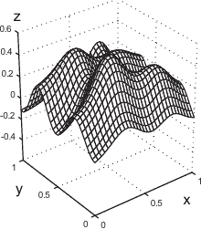
Examples of generated surfaces are given in figure 4.17.
.
Examples of generated surfaces are given in figure 4.17.
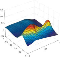
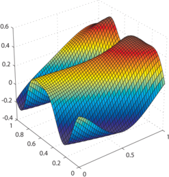
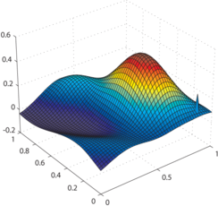
Figure 4.17:
Examples of randomly generated surfaces for the experiments.
|
|
The second type of data we have used in these experiments are real depth maps obtained by stereo imaging means.
Figure 4.18 shows the data.
The range images we have used in these experiments are large: their size is approximately
 pixels.
Therefore, with the approach presented in this section, it is difficult (even impossible) to reconstruct a surface from the original datasets.
This is the reason why the range images have been subsampled over a regular grid of size
pixels.
Therefore, with the approach presented in this section, it is difficult (even impossible) to reconstruct a surface from the original datasets.
This is the reason why the range images have been subsampled over a regular grid of size
 .
However, the full resolution image is used when comparing a reconstructed surface to the initial dataset.
.
However, the full resolution image is used when comparing a reconstructed surface to the initial dataset.
Figure 4.18:
Real range data used in the experiments of this section (Courtesy of Toby Collins). Top row: data represented as a textured 3D surface. Bottom row: same data as in the top row but represented with depth maps.
|
|
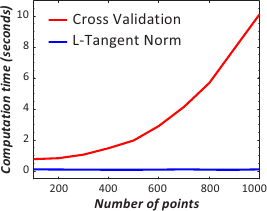
We intend to compare the computation time of the evaluation for a single value of the regularization parameter of the cross-validation score and the L-tangent norm.
To do so, we take a surface and we sample it for several numbers of points.
The timings reported in figure 4.19 have been obtained with the cputime function of Matlab and for the (arbitrary) regularization parameter
 .
Note that the timing for each distinct number of points has been repeated multiple times in order to get stable results.
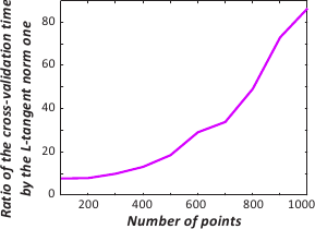
Not surprisingly, figure 4.19 tells us that the evaluation for a single point with the L-tangent norm is far much faster than with cross-validation.
This comes from the fact that the inversion of a matrix is needed in the computation of the cross-validation score while only multiplications between sparse matrices and vectors are involved in the L-tangent norm computation.
.
Note that the timing for each distinct number of points has been repeated multiple times in order to get stable results.
Not surprisingly, figure 4.19 tells us that the evaluation for a single point with the L-tangent norm is far much faster than with cross-validation.
This comes from the fact that the inversion of a matrix is needed in the computation of the cross-validation score while only multiplications between sparse matrices and vectors are involved in the L-tangent norm computation.
Figure 4.19:
Comparison of the cross-validation versus the L-tangent norm computation time for the evaluation of the criteria at a single value. (a) Plot for both cross-validation and the L-Tangent Norm criteria. (b) Ratio of the timings (cross-validation timings divided by the L-Tangent Norm timings).
|
 |
 |
| (a) |
(b) |
|
In this experiment, we are interested in the computation time of the whole optimization process for both the L-tangent norm and cross-validation.
We have taken 300 examples of randomly generated surfaces known through a noisy sampling.
The cross-validation optimization process is performed using a golden section search (implemented in the fminbnd function of Matlab).
The results are shown in figure 4.20.
As in the previous experiment, the optimization of the L-tangent norm is faster than for cross-validation.
Figure 4.20:
Computation time needed to optimize the L-tangent norm and the cross-validation.
|
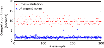 |
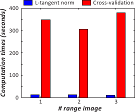
Figure 4.21 shows the computation times needed to the whole surface reconstruction problem with the three range images presented in figure 4.18.
Timings for both the L-tangent norm criterion and the cross-validation score are given in figure 4.21.
As expected, using the L-tangent norm is faster than using cross-validation.
Figure 4.21:
Computation time needed to reconstruct the whole surfaces from the range data of figure 4.18 using the L-tangent norm and cross-validation.
|
 |
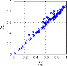
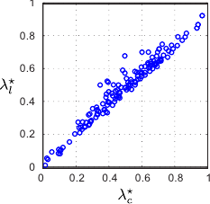
This experiment aims at comparing the regularization parameter obtained with our L-tangent norm and with the cross-validation criterion.
To do so, we have taken noisy samples of randomly generated surfaces.
Then, the regularization parameters obtained with cross-validation (the
 ) for each dataset are plotted versus the regularization parameter determined with the L-tangent norm (the
 ).
The results are reported in figure 4.22.
We see from figure 4.22 that the regularization parameters obtained with the L-tangent norm are often close to the ones obtained with cross-validation.
One can observe that the L-tangent norm tends to slightly under-estimate large regularization parameters.
However, large regularization parameters are usually obtained for datasets with a lot of noise or badly constrained.
In such cases, the accuracy of the regularization parameter does not matter so much.
).
The results are reported in figure 4.22.
We see from figure 4.22 that the regularization parameters obtained with the L-tangent norm are often close to the ones obtained with cross-validation.
One can observe that the L-tangent norm tends to slightly under-estimate large regularization parameters.
However, large regularization parameters are usually obtained for datasets with a lot of noise or badly constrained.
In such cases, the accuracy of the regularization parameter does not matter so much.
In this experiment, we compare the surfaces reconstructed from data obtained as noisy discretizations of randomly generated surfaces.
Let us denote the original randomly generated surface,  ,
,  and
and  the surfaces reconstructed using respectively cross-validation, the L-curve criterion and our L-tangent norm.
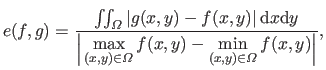
The difference between the original surface and the reconstructed ones is measured with the Integral Relative Error (IRE).
If the functions , , and are all defined over the domain
the surfaces reconstructed using respectively cross-validation, the L-curve criterion and our L-tangent norm.
The difference between the original surface and the reconstructed ones is measured with the Integral Relative Error (IRE).
If the functions , , and are all defined over the domain  , then the IRE is given by:
 |
(4.72) |
where the function  is either , or .
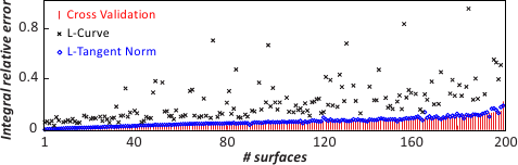
The results of this experiment are reported in figure 4.23.
This figure tells us that the reconstruction errors are small and similar for cross-validation and the L-tangent norm.
The IRE for surfaces reconstructed using the L-curve criterion are much larger than with the two other criteria.
Moreover, only IRE s lower than 1 are reported for the L-curve criterion: the IRE was greater than 1 for 48 test surfaces.
These large IRE s are mainly due to a failure in the maximization of the L-curve criterion.
is either , or .
The results of this experiment are reported in figure 4.23.
This figure tells us that the reconstruction errors are small and similar for cross-validation and the L-tangent norm.
The IRE for surfaces reconstructed using the L-curve criterion are much larger than with the two other criteria.
Moreover, only IRE s lower than 1 are reported for the L-curve criterion: the IRE was greater than 1 for 48 test surfaces.
These large IRE s are mainly due to a failure in the maximization of the L-curve criterion.
Figure 4.23:
Integral relative errors for 200 randomly generated surfaces sampled over 500 points with additive normally-distributed noise.
|
 |
In this last experiment, we intend to compare the surfaces reconstructed from real range images.
To do so, we take again the three range images of figure 4.18.
Let  be the original range image (before subsampling).
Let and be the reconstructed surfaces using respectively the L-tangent norm and the cross-validation criterion to choose the regularization parameter.
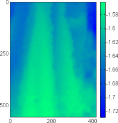
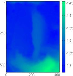
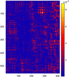
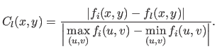
The results of this experiment are presented in the form of Relative Error Maps (REM).
The REM for the surface reconstructed using the L-tangent norm is a picture such that each pixels
be the original range image (before subsampling).
Let and be the reconstructed surfaces using respectively the L-tangent norm and the cross-validation criterion to choose the regularization parameter.
The results of this experiment are presented in the form of Relative Error Maps (REM).
The REM for the surface reconstructed using the L-tangent norm is a picture such that each pixels  is associated to a colour
  proportional to the difference of depth between the reconstructed surface and the original one.
This is written as:
proportional to the difference of depth between the reconstructed surface and the original one.
This is written as:
 |
(4.73) |
The REM for the surface reconstructed using cross-validation,  , is defined similarly to equation (4.74)) except that is replaced by .
We also define the Difference Error Map (DEM) by
, is defined similarly to equation (4.74)) except that is replaced by .
We also define the Difference Error Map (DEM) by
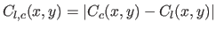 .
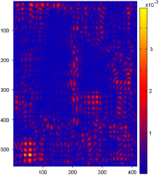
The results of the comparison between surfaces reconstructed from range images using the L-tangent norm and the cross-validation are reported in figure 4.24.
On this figure, only the error map for the L-tangent norm is reported.
Indeed, as it is shown in figure 4.24 (d-f), the two reconstructed surfaces are very similar (which is the point of main interest in this experiment).
Even if the reconstruction errors are not negligible (figure 4.24 (a-c)), they are still small.
The main reason for these errors is the subsampling of the initial datasets.
.
The results of the comparison between surfaces reconstructed from range images using the L-tangent norm and the cross-validation are reported in figure 4.24.
On this figure, only the error map for the L-tangent norm is reported.
Indeed, as it is shown in figure 4.24 (d-f), the two reconstructed surfaces are very similar (which is the point of main interest in this experiment).
Even if the reconstruction errors are not negligible (figure 4.24 (a-c)), they are still small.
The main reason for these errors is the subsampling of the initial datasets.
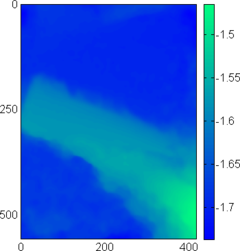
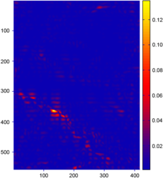
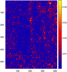
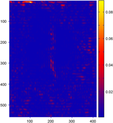
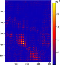
Figure 4.24:
(a-c) Relative error maps (REM) for the surfaces reconstructed using the L-tangent norm criterion for the three range images of figure 4.18. (d-f) Difference error maps (DEM) between the surfaces reconstructed using the L-tangent norm criterion and the cross-validation criterion.
|
|
Contributions to Parametric Image Registration and 3D Surface Reconstruction (Ph.D. dissertation, November 2010) - Florent Brunet
Webpage generated on July 2011
PDF version (11 Mo)