BleamCard: the first augmented reality card. Get your own on Indiegogo!
Subsections
Hyperparameters
In this section, we discuss an important aspect of parameter estimation problems: the hyperparameters.
This section is organized as follows.
We first try to give a general definition of what the hyperparameters are.
Since the distinction between classical parameters and hyperparameters is somewhat unclear, the general definition is then complemented with a simple practical example which allows one to get a good grasp at this concept.
We finish this section with an explanation of the common approach to determine automatically hyperparameters.
The principle will come along with a review of the most common and practical approaches used to determine hyperparameters.
Note that the problems induced by the hyperparameters are one of the central topics tackled in this thesis.
Consequently, more advanced aspects on hyperparameters, including our contributions, will be spread across this document.
Table 3.3 synthesizes the parts of this document in which hyperparameters are involved.
Table 3.3:
Parts of this thesis that deal with hyperparameters.
|
| Where |
What |
| 3.2 |
Definition, description, and common tools. |
| 4.2 |
The L-Tangent Norm: a contribution that allows one to tune hyperparameters for range surface fitting |
| 4.2.2 |
Review of another approach to determine hyperparameters: the L-curve criterion |
| 4.3.1.4 |
Another approach to determine hyperparameters specific to range surface fitting adapted from the Morozov's discrepancy principle |
| 5.3 |
One of our contribution that uses the specific setup of feature-based image registration to automatically tune hyperparameters |
|
As it was explained in the previous sections, the goal of parameter estimation is to find the natural parameters of a parametric model.
The natural parameters are, to cite a few, the coefficients of a polynomial, the weights of a B-spline or the control points of a NURBS.
Generally, in such problems, one also has to determine `extra-parameters' which are, for instance, a value controlling the configuration of the parametric model or a parameter of a prior distribution in a MAP estimation scheme.
This supplemental parameters are called the hyperparameters.
In other words, an hyperparameter is a parameter of a prior (as distinguished from the parameters of the model for the underlying system under analysis).
For example, the degree of a B-spline is an hyperparameter.
The number of knots of a B-spline is another example of hyperparameter linked to the parametric model itself.
The weight given to a regularization term in a cost function is also an hyperparameter (linked to the cost function instead of the parametric model of function).
In order to make things clearer, we now illustrate the concept of hyperparameter on a simple example.
It will allow us to show how some usual types of hyperparameters arise in a parameter estimation problem.
Let us consider that we have a set of data points
 with
with
 and
and
 .
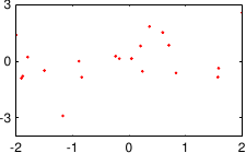
These data are illustrated in figure 3.4.
.
These data are illustrated in figure 3.4.
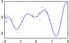
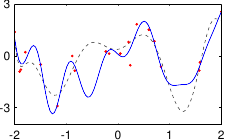
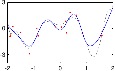
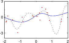
Figure 3.4:
Noisy data to fit with a polynomial.
|
 |
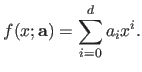
We now consider the problem of fitting a polynomial of degree  to this data set.
The parametric model to use is a function
to this data set.
The parametric model to use is a function  from
from
 to
to
 that can be written as:
 |
(3.28) |
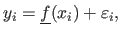
Let us further assume that the data points are noisy and that the errors are normally-distributed with zero mean and standard deviation  .
If we note
.
If we note
 the true function, then we have that:
 |
(3.29) |
where
 for all
 .
One may also want to make an assumption on the fitted polynomial.
For instance, smooth polynomial could be preferred.
This kind of assumption is quite usual since it helps in compensating the undesirable effects caused by for instance, noise, outliers, or lack of data.
In the MAP estimation framework, this can be achieved using a prior distribution on the parameters.
For example, we could say that smooth polynomials (i.e. the ones that minimizes the bending energy) must be more probable than other ones.
This can be implemented using the following prior distribution on the parameters:
.
One may also want to make an assumption on the fitted polynomial.
For instance, smooth polynomial could be preferred.
This kind of assumption is quite usual since it helps in compensating the undesirable effects caused by for instance, noise, outliers, or lack of data.
In the MAP estimation framework, this can be achieved using a prior distribution on the parameters.
For example, we could say that smooth polynomials (i.e. the ones that minimizes the bending energy) must be more probable than other ones.
This can be implemented using the following prior distribution on the parameters:
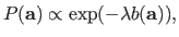 |
(3.30) |
where  is the function from
 to
to
 that gives the pseudo-bending energy of the polynomial:
 |
(3.31) |
where
 is the definition domain of the polynomial with respect to the free variable
  .
The PDF of the prior distribution defined in figure 3.30 is a bell-shaped curve which width is controlled by the parameter
.
The PDF of the prior distribution defined in figure 3.30 is a bell-shaped curve which width is controlled by the parameter
 .
A large
.
A large  results in a narrow bell-shaped curved which means that only very smooth polynomials will have a non-negligible probability.
On the contrary, a small lambda produces a large bell-shaped curve which makes probable rugged polynomials.
The prior parameter is often named the smoothing parameter or regularization parameter.
If we apply the MAP principles (as described in section 3.1.1.5) with the hypothesis we have just made, then estimating the coefficients
results in a narrow bell-shaped curved which means that only very smooth polynomials will have a non-negligible probability.
On the contrary, a small lambda produces a large bell-shaped curve which makes probable rugged polynomials.
The prior parameter is often named the smoothing parameter or regularization parameter.
If we apply the MAP principles (as described in section 3.1.1.5) with the hypothesis we have just made, then estimating the coefficients
 of the polynomial is equivalent to solve the following minimization problem:
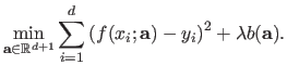 |
(3.32) |
In equation (3.32), the coefficients of the vector
are the natural parameters of the estimation problem while the values and are the hyperparameters.
More precisely, the degree is a model hyperparameter since it is a parameter that `tune' the underlying model of function.
The value is what we call a cost hyperparameter since it is linked to the cost function itself.
If we consider that and are given, then problem (3.32) is a simple linear least-squares problem.
However, determining correct values for the hyperparameters is a difficult task, especially if we want this determination to be automatic.
It is nonetheless mandatory in order to get proper results.
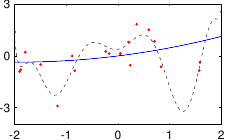
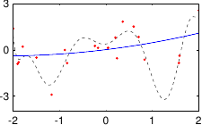
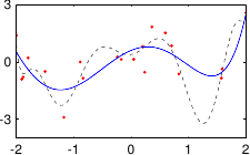
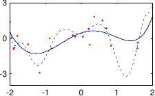
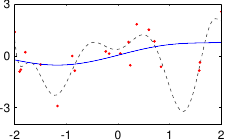
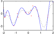
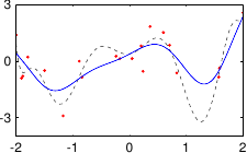
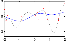
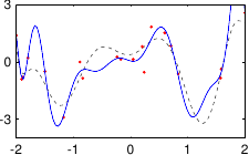
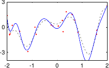
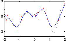
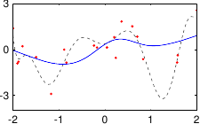
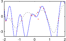
Figure 3.5 shows the influence of the hyperparameters and of our example with the data of figure 3.4.
A fact that makes difficult the automatic computation of the hyperparameters is that they cannot be directly included in the initial optimization problem.
For instance, in the context of our example, the following minimization problem will not lead to the expected results:
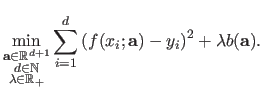 |
(3.33) |
For instance, the bending term is a positive value.
Consequently, the best way to minimize the influence of this term in the cost function of equation (3.33) is to set
 .
This is clearly not the expected result since, for some reasons, we wanted a `smoothed' polynomial.
The same kind of dubious effect will arise for the degree of the polynomial.
Indeed, the error in equation (3.33) will be completely minimized (i.e. the value of the cost function is null) if the fitted polynomial interpolates the data points.
This is achieved by taking
.
This is clearly not the expected result since, for some reasons, we wanted a `smoothed' polynomial.
The same kind of dubious effect will arise for the degree of the polynomial.
Indeed, the error in equation (3.33) will be completely minimized (i.e. the value of the cost function is null) if the fitted polynomial interpolates the data points.
This is achieved by taking  where
where  is the number of data points.
In our example, we had 25 data points but the best fit is realized with a polynomial of degree 10.
The general principles used to build a correct approach for automatic hyperparameter selection will be explained in section 3.2.2.
is the number of data points.
In our example, we had 25 data points but the best fit is realized with a polynomial of degree 10.
The general principles used to build a correct approach for automatic hyperparameter selection will be explained in section 3.2.2.
Formal Definitions
We give here a set of definitions which are more or less3.4 related to the hyperparameters.
In this thesis, we classify the hyperparameters into two main categories.
First, we consider the parameters linked to the prior distribution given to the natural parameter to estimate.
We call this type of hyperparameters the cost hyperparameters since, after having derived an estimation procedure with, for instance with MAP, they appear as tuning values of the cost function.
Second, we consider the model hyperparameters which are directly linked to the parametric model of function.
Examples of this second type of hyperparameter include the degree of a polynomial or of a B-spline, the number of control points of a B-spline, the kernel bandwidth of a RBF, the number of centres of a RBF, etc.
Roughly speaking, the (effective) complexity of a parametric model corresponds to its number of degrees of freedom minus the `number'3.5 of constraints implicitly induced by the prior given to the parameters of the model.
Consequently, the complexity of a parametric model is mostly tuned by the hyperparameters.
In order to get a correct parametric estimator, the complexity of the model must meet the actual complexity carried by the data.
By `actual', we mean the complexity of the data excluding the noise.
In practice, this actual complexity is generally not known precisely.
Indeed, given a set of data, it is hard to distinguish between the noise and the true information.
This fact systematically leads to problems such as underfitting and overfitting which are closely related to the concepts of bias and variance of an estimator.
These concepts are explained in the next paragraphs along with some other definitions.
The residual error is the sum of the errors between the estimated parametric model and the data (at the location of the data points).
For a parametric model and a set of parameters
 , the residual error may be defined as:
 |
(3.34) |
where is a function that gives the distance between its two arguments (for instance, a common choice is the squared Euclidean norm).
Note that equation (3.34) is similar to what is generally minimized in a parameter estimation problem.
However, as it will be seen later, having a minimal residual error does not always lead to the proper results.
The prediction error (also known as the expected prediction error or generalization error or test error) is a quantity that measures how well an estimated model is able to generalize (96).
Given a point  different of the points used to estimate the parameters, the prediction error measure the difference between the estimated value
 and the true value
 .
In other words, it measures how well the estimated model performs, i.e. how close it is to the true function.
The prediction error at is given by:
.
In other words, it measures how well the estimated model performs, i.e. how close it is to the true function.
The prediction error at is given by:
![$\displaystyle E \left [ \left ( \underline{f}(x_0) - f(x_0 ; \mathbf{p}) \right )^2 \right ]$](img703.png) |
(3.35) |
The prediction error can be broken down into two terms:
![$\displaystyle \left ( E\left [ f(x_0 ; \mathbf{p}) \right ] - \underline{f}(x_0) \right )^2 + \mathrm{Var}(f(x_0 ; \mathbf{p})).$](img704.png) |
(3.36) |
The first term is the squared bias of the estimator while the second term is the variance of the estimator.
Equation (3.36) should ideally be the cost function to be minimized for parameter estimation but this is not possible in practice because
is not known.
A parametric model with low complexity leads to a high bias and low variance.
On the contrary, a parametric model with high complexity leads to a low bias and high variance.
This is called the bias-variance compromise.
Note that minimizing usual cost functions, which are particular forms of Equation (3.34), is equivalent to minimize only the bias term in equation (3.36).
This is the reason why the hyperparameters cannot be directly included in the standard optimization problem for parameter estimation since it would only reduce the bias of the estimator, not its variance.
The phenomena of underfitting and overfitting are closely related to the bias-variance compromise.
The underfitting problem arises when the complexity of the parametric model is not enough high.
In other words, the parametric model is not flexible enough to model the data.
It corresponds to an estimator with high bias and low variance.
On the other side, there is the overfitting problem.
It corresponds to a parametric model with a too high level of complexity.
In this case, it is so flexible that the estimated parametric model will model not only the data but also the noise.
It is an estimator with high variance and low bias.
An estimated parametric model is said to interpolate the data
if we have that:
 |
(3.37) |
It corresponds to the estimator with minimal bias.
If the data point are noisy (as it is always the case in the real world), it also corresponds to the estimator with maximal variance.
Consequently, interpolators are generally not the best estimators (at least, when there is noise in the data).
It is thus preferable to have estimators that approximates the data instead of interpolating them, i.e. such that:
 |
(3.38) |
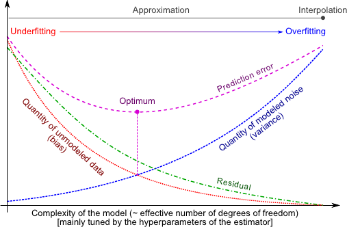
Figure 3.6:
Illustration of the concepts presented in section 3.2.1.2. The hyperparameters in an estimation scheme (both cost and model hyperparameters) allows one to tune the complexity of a parametric model. The best hyperparameters for an estimator are the one that would result in a minimization of the prediction error (purple line). The prediction error cannot be computed in practice since its definition relies on the knowledge of the true underlying function. Instead, one generally minimizes a quantity related to the residual error (green line). This quantity is closely related to the bias of the estimator. Minimizing the bias of an estimator is not sufficient enough since it may lead to a fitted function that model the noise.
|
 |
Automatic Computation of the Hyperparameters
As we just explained, the hyperparameters are important in order to estimate proper parameters.
We also said that determining correct hyperparameters was not a simple problem in the sense that it cannot be directly included in the minimization problem derived to estimate the natural parameters.
It is nonetheless possible to use automatic procedure to determine the hyperparameters.
In fact, there exists an incredibly large number of such procedures.
For that matter, some of the contributions we propose in this document are new ways of automatically determining hyperparameters.
The most general approach to automatically determine hyperparameters (in other words, to select the model complexity) consists in minimizing an external criterion which, in a nutshell, assesses the quality of the estimated model.
Let us call  this criterion.
In the general case, is a function from
this criterion.
In the general case, is a function from
 to
where
to
where  is the number of hyperparameters (which are grouped in a vector denoted
 in this section).
Always in the general case,
in this section).
Always in the general case,
 is small when the function induced by the hyperparameters
 (and the subsequent parameters) is correct, i.e. it does not underfit nor overfit the data.
Let
(and the subsequent parameters) is correct, i.e. it does not underfit nor overfit the data.
Let  be the cost function used to determine the natural parameters of a model from the data.
For the needs of this section, we consider as a function of both the natural parameters and the hyperparameters.
In particular, is a function from
be the cost function used to determine the natural parameters of a model from the data.
For the needs of this section, we consider as a function of both the natural parameters and the hyperparameters.
In particular, is a function from
 where is the number of natural parameters and is the number of hyperparameters.
The general principle of parameter estimation with automatic hyperparameters selection is to solve the following nested optimization problem:
where is the number of natural parameters and is the number of hyperparameters.
The general principle of parameter estimation with automatic hyperparameters selection is to solve the following nested optimization problem:
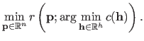 |
(3.39) |
Note that the problem stated in equation (3.39) is quite different of the inconsistent problem in which both the parameters and the hyperparameters are mixed in the initial optimization problem:
 |
(3.40) |
Indeed, for the reasons explained above, the solution of problem (3.40) would be the one with minimal bias and, consequently, it would completely overfit the data (if possible, it will even try to interpolate the data instead of finding an appropriate approximation).
Given what was just said, the main difficulty for building an automatic hyperparameter selection procedure is obviously to find a criterion which reach a minimum value for correct hyperparameters3.6.
Of course, the best choice for would be the prediction error but, unfortunately, it is not possible since this criterion relies on an unknown: the true function.
Many criteria have been proposed.
They take their root in different domain: information theory, Bayesian reasoning, philosophy, etc.
We review some of the most classical ones in the next sections.
Cross-Validation is one of the most common approach to automatically tune hyperparameters.
At a glance, the principle of Cross-Validation is to build a criterion that, for a given set of hyperparameters, measures how well the resulting estimated model is able to generalize the data.
In other words, it measures how good the behaviour of the estimated model is `between' the data.
Of course, the ability to generalize of an estimated model can be computed precisely only if the true function is available.
The magic of Cross-Validation is to be able to estimate this ability only from the data and without requiring the true model.
The general principle of Cross-Validation relies on an approach commonly used in learning theory: dividing the dataset into several subsets.
Each one of these subsets is then alternatively used as a training set or as a test set to build Cross-Validation score function.
The way the dataset is divided gives rise to different variant of Cross-Validation.
In some special cases, efficient approximations can be derived which make computations faster.
In the next paragraphs, we review some of the most common flavour of Cross-Validation.
Cross-validation is very interesting for several reasons (6).
In particular, it is `universal' in the sense that the data splitting technique is very generic.
The only assumption to be made for using cross-validation is that the data must be identically distributed.
Besides, it is not linked to a particular framework as most as other methods for hyperparameters selection are.
For instance, Mallow's  is only applicable for least-squares cost functions (see section 3.2.2.3).
Leave-one-out Cross-Validation (LOOCV) is one of the simplest variant of the general Cross-Validation principle.
A detailed study of LOOCV is available in (193).
For a given set of hyperparameters
, let
 be the parameters of the model estimated from the data with the
  th data point left out.
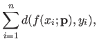
The LOOCV criterion is defined as:
th data point left out.
The LOOCV criterion is defined as:
 |
(3.41) |
where is the function that gives the discrepancy between its two arguments.
For instance, it may be the squared Euclidean norm.
Equation (3.41) means that every point of the initial dataset is used as a validation set for the model estimated from the other data points.
If there are enough points in the data set (say, for instance,  ) then it is reasonable to think that the parameters estimated with
  points are close to the ones that would be estimated with all the initial points.
Consequently, for a given ,
points are close to the ones that would be estimated with all the initial points.
Consequently, for a given ,
 is a good approximation of the generalization error made at
  .
Therefore,
.
Therefore,
 is an approximation of the generalization error resulting of the given set of hyperparameters
.
is an approximation of the generalization error resulting of the given set of hyperparameters
.
LOOCV is quite appealing and often gives satisfactory results in practice.
However, as one may notice from equation (3.41), it can be extremely heavy to compute.
Indeed, each term of the sum in equation (3.41) requires one to estimate the set of parameters
.
If is large then the sum in equation (3.41) has many terms, each one of which being potentially long to compute.
In the case where the cost function is a sum of squared linear terms (which happens if the parametric model is linear with respect to its parameters and if the noise is assumed to be normally distributed), a closed-form non-iterative approximation of the LOOCV criterion exists.
The general form of a linear least squares parameter estimation problem is:
 |
(3.42) |
where
 is a vector containing the right part of the measurement (the
  for
). The matrix
for
). The matrix
 is a matrix that depends on the left part of the measurements (the
 for
), on the parametric model of function, and on the hyperparameters
.
The solution
for
), on the parametric model of function, and on the hyperparameters
.
The solution
 of problem (3.42) is given by:
 |
(3.43) |
Note that
depends on the hyperparameters
(which are considered to be given and fixed in equation (3.43)).
The hat matrix, denoted
 , is the matrix of the linear application that maps the measurements to the values predicted by the estimated model (denoted
  for
and gathered in a vector
for
and gathered in a vector
 ).
It is defined by:
).
It is defined by:
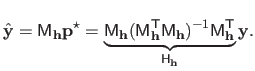 |
(3.44) |
The closed-form approximation to the LOOCV criterion, denoted
 , is given by:
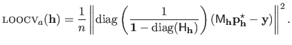 |
(3.45) |
From equation (3.45), we see that for a given set of hyperparameter
, the computational complexity of the criterion
is reduced by one order of magnitude compared to the exact but iterative criterion LOOCV.
A proof of the derivation of the
criterion as an approximation of the LOOCV criterion can be found in, for instance, (193,79,12).
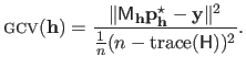
Generalized Cross-Validation (GCV) is a variation of the
criterion proposed in (51).
It consists in replacing the individual diagonal coefficients of the hat matrix in equation (3.45) by the average of all the coefficients of the diagonal.
The GCV criterion is thus defined as:
 |
(3.46) |
The GCV criterion was originally proposed to reduce the computational complexity but it has been found that this criterion possesses several interesting properties.
In particular, it has been shown (85) that the GCV criterion is an approximation of Mallow's criterion (see section 3.2.2.3).
It has also been shown to be rotation-invariant approximation of the PRESS (PREdiction Sum of Squares) statistic of Allen3.7.
Leave- -out Cross-Validation (LPOCV) (174) is another variant of the Cross-Validation principle.
It is similar to the LOOCV in the sense that it uses an exhaustive data splitting strategy.
With the `basic' LOOCV, all the possible subsets of size 1 were alternatively used as test sets.
With the LPOCV, every possible subset of size (with fixed and chosen in
-out Cross-Validation (LPOCV) (174) is another variant of the Cross-Validation principle.
It is similar to the LOOCV in the sense that it uses an exhaustive data splitting strategy.
With the `basic' LOOCV, all the possible subsets of size 1 were alternatively used as test sets.
With the LPOCV, every possible subset of size (with fixed and chosen in
 ) is successively used as a test set.
Of course, the computational burden of such an approach is potentially gigantic since there are
) is successively used as a test set.
Of course, the computational burden of such an approach is potentially gigantic since there are
 subsets of size in a set of size .
Note that if
subsets of size in a set of size .
Note that if  then LPOCV is equivalent to LOOCV.
Another common flavour of the Cross-Validation principle is the  -fold Cross-Validation (VCV).
It was introduced by (77) as an alternative to the computationally expensive LOOCV.
A full review of the VCV can be found in (27).
(6) gives some useful insight about the VCV.
Again, the initial dataset is split into training and test sets.
However, contrarily to LOOCV and LPOCV, the VCV is not an exhaustive approach.
In the VCV case, the dataset is split into subsets of approximately equal size.
These subsets form a partition of the initial dataset.
This splitting is done before the computation of the criterion and does not vary after that.
Each subset is then used alternatively used as a test set.
Given a set of hyperparameters
, let
-fold Cross-Validation (VCV).
It was introduced by (77) as an alternative to the computationally expensive LOOCV.
A full review of the VCV can be found in (27).
(6) gives some useful insight about the VCV.
Again, the initial dataset is split into training and test sets.
However, contrarily to LOOCV and LPOCV, the VCV is not an exhaustive approach.
In the VCV case, the dataset is split into subsets of approximately equal size.
These subsets form a partition of the initial dataset.
This splitting is done before the computation of the criterion and does not vary after that.
Each subset is then used alternatively used as a test set.
Given a set of hyperparameters
, let
![$ \mathbf{p}^{[v]}_{\mathbf{h}}$](img738.png) be the set of parameters obtained from the data with the
be the set of parameters obtained from the data with the  th subset left out.
Let
th subset left out.
Let  be the size of the th subsets.
The VCV criterion is defined by:
be the size of the th subsets.
The VCV criterion is defined by:
![$\displaystyle \textsc{vcv}\xspace (\mathbf{h}) = \sum_{v=1}^V \frac{m_v}{n} \su...
...m_v} d\left (y_k,f \left ( x_k ; \mathbf{p}_{\mathbf{h}}^{[v]}\right )\right ),$](img741.png) |
(3.47) |
where is a function that measures the difference between its two arguments (for instance, the squared Euclidean norm).
In practice, the number of subsets used for computing the VCV is often chosen as
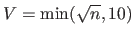 .
This gives a good trade-off between accuracy of the approximation of the generalization error and the computational burden.
Although very appealing, our experience leads us to say that the VCV criterion does not give results as good as the ones obtained with the LOOCV or the GCV.
.
This gives a good trade-off between accuracy of the approximation of the generalization error and the computational burden.
Although very appealing, our experience leads us to say that the VCV criterion does not give results as good as the ones obtained with the LOOCV or the GCV.
The list of cross-validation criteria we presented so far is not even close to being exhaustive.
We will not detail here all the variant.
For the sake of the culture, we will just cite a few of them: Gauss-Newton leave-one-out cross-validation (66), balanced incomplete cross-validation, repeated learning-testing, Monte-Carlo cross-validation, bias-corrected cross-validation, etc.
Note that (6) gives a good overview on some of these cross-validation criteria.
Mallow's
Introduced in (120), Mallow's is a criterion that can be used to automatically tune hyperparameters.
The validity of this criterion is limited to linear least squares estimators.
Besides, it is designed to work with one integer hyperparameter.
For the sake of simplicity, let us consider that the model is a polynomial and that the only hyperparameter is the degree of this polynomial.
Let us further assume that  is the maximal degree allowed for the polynomial (i.e.
 ).
Mallow's is given by:
).
Mallow's is given by:
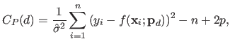 |
(3.48) |
where is the number of parameter of the model induced by the hyperparameter ( in the case of a polynomial),
 is the maximum likelihood estimate of the parameters given the hyperparameter , is the number of data points, and
 is an estimate of the error variance that is usually computed as the residual sum of squares with the full model (in this case, with a polynomial of degree ).
Other criteria based on the initial Mallows criterion have been proposed.
For instance, robust versions of Mallow's criterion are proposed in (160,159).
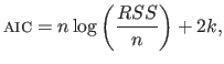
Akaike Information Criterion (AIC) is a criterion that relies on information theoretic foundations.
It was introduced in (2).
Useful insights on AIC are given in (79,41).
In this section, we give the basic elements that allows one to progressively build the AIC criterion.
The AIC criterion will finally be given in equation (3.56).
The Kullback-Leibler (K-L) divergence is the quantity defined as:
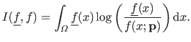 |
(3.49) |
It may be seen as a `distance'3.8 between the true model
and the estimated model
 .
The K-L divergence cannot be used directly as a criterion to choose the hyperparameters since it would require one to know the true model.
Therefore, the selection criterion will aim at minimizing an expected estimated K-L divergence:
.
The K-L divergence cannot be used directly as a criterion to choose the hyperparameters since it would require one to know the true model.
Therefore, the selection criterion will aim at minimizing an expected estimated K-L divergence:
![$\displaystyle E_y[I(\underline{f},f)].$](img751.png) |
(3.50) |
The K-L divergence may rewritten as:
For varying hyperparameters, the first term in equation (3.52) is a constant, and therefore:
![$\displaystyle I(\underline{f},f) = c - E[\log(f(x ; \mathbf{p}))].$](img755.png) |
(3.53) |
The second term in equation (3.52) is the relative Kullback-Leibler divergence.
In order to get a practical criterion, the relative K-L need to be approximated (because it still depends on
).
This is the goal of AIC:
![$\displaystyle \max E_y E_x[\log(f(x ; \mathbf{p}))].$](img756.png) |
(3.54) |
Akaike's work says that an approximately unbiased estimate of
![$ \max E_y E_x[\log(f(x ; \mathbf{p}))]$](img757.png) is:
is:
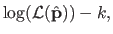 |
(3.55) |
with
 the likelihood function,
 the maximum likelihood estimate of
, and the number of parameters.
The AIC is given by:
the maximum likelihood estimate of
, and the number of parameters.
The AIC is given by:
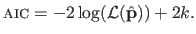 |
(3.56) |
The terms in equation (3.56) can be identified to the terms in the bias-variance trade-off: the first term corresponds to the bias while the second term corresponds to the variance.
If the errors are assumed to be i.i.d. normally-distributed, the AIC can be expressed by:
 |
(3.57) |
where
 .
.
Although theoretically founded, several improvement and variations have been built upon the AIC.
For instance, if the sample size is small with respect to the number of parameters, then it is preferable to use the corrected AIC given by (180):
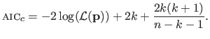 |
(3.58) |
The Bayesian Information Criterion (BIC) is another criterion that can be used to automatically tune hyperparameters.
It was proposed by (171).
The BIC is defined as follows:
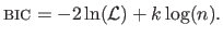 |
(3.59) |
Equation (3.59) shows that BIC is very similar to the AIC.
The practical difference between these two criteria is that BIC tends to penalize complex models more heavily than AIC (because the second term in equation (3.59) depends on the number of model parameters).
The other major difference between AIC and BIC is that BIC is motivated in a quite different way than AIC.
To this matter, and as noticed in (41), the name BIC is a bit misleading since this criterion does not rely on information theory but, instead, on a Bayesian approach to model selection.
A synthetic explanation of the BIC foundations is given in (96, §7.7).
We now give a quick justification of the BIC.
Let  be the set of models generated by all the possible hyperparameters, i.e. :
 |
(3.60) |
where
 is the parametric model (in which we write explicitly the dependency on the hyperparameters
).
The goal is to find the best element in the set of functions .
Let us assume that we have a prior distribution
is the parametric model (in which we write explicitly the dependency on the hyperparameters
).
The goal is to find the best element in the set of functions .
Let us assume that we have a prior distribution
 of the parameters of each model in .
The posterior probability of a given model is given by:
of the parameters of each model in .
The posterior probability of a given model is given by:
where
 represents the data.
If one wants to compare the relative quality of two set of hyperparameters
and
represents the data.
If one wants to compare the relative quality of two set of hyperparameters
and
 , he can look at the ratio of their posterior probability:
 |
(3.63) |
If the ratio in equation (3.63) is greater than one, the model induced by the hyperparameters
is considered to be better than the one induced by the hyperparameters
.
It is a reasonable assumption to consider that the prior distribution of the models is uniform.
Consequently, the first factor in equation (3.63) is just a constant.
The second factor (known as the Bayes factor) can be approximated using this identity (96):
 |
(3.64) |
where
 is the maximum likelihood estimate of the parameters given the hyperparameters and
 is the number of free parameter in
 .
This last equation is equivalent to the BIC.
Consequently, choosing the hyperparameters that give the minimum BIC is equivalent to maximize the (approximate) posterior probability.
.
This last equation is equivalent to the BIC.
Consequently, choosing the hyperparameters that give the minimum BIC is equivalent to maximize the (approximate) posterior probability.
The Minimum Description Length (MDL) criterion is another criterion that can be used to determine automatically hyperparameters.
It was first introduced by (155) and it relies on information theory.
A good synthesis of the underlying principles of MDL are given by (132,131).
In a nutshell, MDL is a formal implementation of the well known principle of the Occam's razor which states that ``entities must not be multiplied beyond necessity''3.9.
In other words, if several models can explain the same set of data, the simplest is most likely to be the correct one.
Although appealing, this philosophical principle should be considered with extreme care, especially because the notion of `simplest' is quite unclear.
Without care, it is virtually possible to consider as the simplest any set of hyperparameters.
The formal definition of the MDL criterion is actually exactly the same3.10 than the definition of the BIC, i.e. :
 |
(3.65) |
The fundamental difference between BIC and MDL lies in their theoretical roots.
Indeed, MDL relies on information theory and, in particular, the Kolmogorov complexity.
The Kolmogorov complexity, also known as the algorithmic complexity or Turing complexity, is a concept that was independently developed by (179,108,46).
In a nutshell, it measures the complexity of a message (which can be seen as a particular way of describing a parametric model) as the length of the minimal Turing machine that generates this same message.
Unfortunately, the Kolmogorov complexity cannot be calculated because it is related to the famous halting problem which was proven by (187) to be incomputable.
Fortunately, a famous theorem due to (173) gives a lower bound for the Kolmogorov complexity:
![$\displaystyle E[\mathrm{len}(z)] \geq -\int P(z) \log_2(z) \mathrm d z,$](img778.png) |
(3.66) |
where
 is the length of the binary string encoding the continuous random variable
  of distribution
  .
A consequence of this theorem is that encoding a continuous random variable of distribution requires approximately
.
A consequence of this theorem is that encoding a continuous random variable of distribution requires approximately
 bits of information3.11.
We replace the binary logarithm by the
bits of information3.11.
We replace the binary logarithm by the  function since the only difference is an unimportant multiplicative constant.
Let us now consider the dataset made of the inputs
function since the only difference is an unimportant multiplicative constant.
Let us now consider the dataset made of the inputs
 and of the outputs
 .
The required length for encoding
.
The required length for encoding  is the sum of the length required to encode the parameters of a model and of the length required to encode the discrepancy between the true model and the actual measurement, i.e. :
 |
(3.67) |
The first term is the negative logarithm of the posterior probability while the second term is the average length for encoding the parameters.
(155) postulated from results by (173) that the length of the code for
was
 for each parameter, hence the final expression of MDL.
Minimizing the MDL criterion is therefore equivalent to determine the simplest representation of the data, which is why MDL is considered as a formal implementation of the Occam's razor principle.
for each parameter, hence the final expression of MDL.
Minimizing the MDL criterion is therefore equivalent to determine the simplest representation of the data, which is why MDL is considered as a formal implementation of the Occam's razor principle.
In addition to the very generic and widely spread criteria presented in the previous section to automatically compute hyperparameters, there exists others more specific (and generally less-known) approach to determine hyperparameters.
Some of these criteria (such as the L-curve or the Morozov's discrepancy principle) will be used in this document.
Given their lack of generality, we do not review them in this section.
Instead, we will detail them when appropriate in the document.
Although it is not a founded approach, it appears that one of the most common technique to determine hyperparameters is probably to give them some empirical value determined by hand.
A very popular choice is the value 1.
This is what we call, with a bit of irony we must admit, the ` approach'.
Note that this trivial approach has been proved to give reasonable results in many problems (at least with appropriately chosen instances of these problems).
This is probably why a lot of researchers do not believe that the determination of the hyperparameters is a problem of interest.
In our work, we beg to differ and we will, as much as possible, give details on how hyperparameters are chosen.
approach'.
Note that this trivial approach has been proved to give reasonable results in many problems (at least with appropriately chosen instances of these problems).
This is probably why a lot of researchers do not believe that the determination of the hyperparameters is a problem of interest.
In our work, we beg to differ and we will, as much as possible, give details on how hyperparameters are chosen.
Another common approach is to determine typical values for the hyperparameters by looking at the results of extensive experiments.
This type of approach has been used in, for instance, (149,146).
Even though the exact way in which hyperparameters are selected is not always mentioned in scientific papers, we can imagine that most authors use extensive experimentations to determine typical values.
Note that, sometimes, `typical values' do not exist.
This is the case when there exists an important variability between instances of the same problem.
For instance, it is not reasonable to consider that there exists a set of typical hyperparameters for range surface fitting (see chapter 4).
Indeed, in this case, the choice of the hyperparameters heavily relies on the shape of the observed scene.
Contributions to Parametric Image Registration and 3D Surface Reconstruction (Ph.D. dissertation, November 2010) - Florent Brunet
Webpage generated on July 2011
PDF version (11 Mo)