Subsections
In this section, we present some other contributions we made in the topic of reconstructing range surface.
In the previous sections, we considered arbitrary range data in the sense that the locations of the data points did not follow any particular pattern.
In this section, we consider data sets with points arranged on a regular grid.
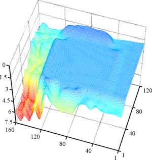
More precisely, we consider data sets in form of depth maps produced by TOF cameras.
This type of data is particularly challenging for several reasons.
Firstly, there is an important amount of data.
With the equipment we used, there was typically around 20 thousands points per depth map.
Secondly, there is usually an important amount of noise in the TOF data.
Besides, this noise is heteroskedastic which means that the variance of the noise is not identical for all the pixels of the depth map.
Thirdly, as TOF cameras can capture data from arbitrary parts of the environment, the resulting depth maps are likely to contain discontinuities.
The contributions proposed in this section aim at coping with these different aspects of TOF data.
This section is organized as follows.
First, we specialize the general approach to range surface fitting with B-splines to the particular case of data arranged on a regular grid.
In this first part, we will just consider an homoskedastic noise.
In addition to the presentation of the general way of handling grid data, we make two contributions: a new regularization term that approximate the bending energy while being compatible with the grid approach and a new manner of selecting the regularization parameter.
Next, we present our multi-step approach for handling heteroskedastic noise and discontinuities.
Finally, the efficiency of our approach is illustrated with a set of experiments.
Fitting a B-spline on Mesh Data
As it will be shown later, fitting a B-spline on mesh data leads to formulas that heavily relies on the Kronecker product.
We thus give here a list of interesting properties linked to the Kronecker product.
The following identities are taken from (61):
Here comes additional properties that will be useful in the derivations of the principles for fitting a B-spline to mesh data:
In this section, we consider that the data set is made of range data points organized as a regular grid of size
 .
This type of data naturally arises with TOF cameras since this device produces depth maps.
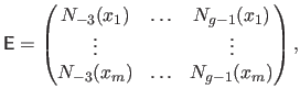
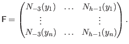
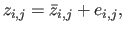
This particular data structure leads to write the whole data set in the following way:
.
This type of data naturally arises with TOF cameras since this device produces depth maps.
This particular data structure leads to write the whole data set in the following way:
 |
(4.88) |
The depths  are grouped in a matrix
 .
.
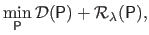
The general principle for fitting a B-spline to mesh range data is the same as the one used in the previous sections.
It is still formulated as a minimization problem with a cost function composed of two terms.
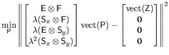
However, for the needs of this section, this optimization problem is formulated in a slightly different way:
 |
(4.89) |
where
 and
and
 are respectively the data term and the regularization term.
Here, we consider that the regularization parameter
are respectively the data term and the regularization term.
Here, we consider that the regularization parameter  is part of the regularization term itself.
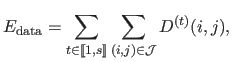
The data term is again defined as the mean squared residual:
 |
(4.90) |
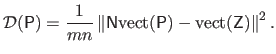
The fact that the data are arranged on a grid is exploited in the collocation matrix
 .
Indeed, since we use uniform cubic B-splines, this matrix is initially defined as:
.
Indeed, since we use uniform cubic B-splines, this matrix is initially defined as:
 |
(4.91) |
From equation (4.92), it is easy to see that the collocation matrix
can be written as the Kronecker product of two matrices:
 |
(4.92) |
where:
 |
(4.93) |
and
 |
(4.94) |
Consequently, the data term can be written as:
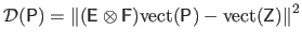 |
(4.95) |
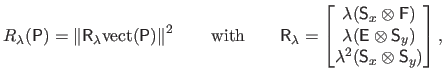
In order to obtain the best efficiency in terms of computational complexity, we propose a new regularization term.
It is a variation of the classical bending energy used so far.
We propose a new regularization term because the classical bending energy cannot be expressed with a tensor product expression.
We define it as:
The main advantage of the regularization term of equation (4.97) is that, as the data term, it can be written using the Kronecker product.
Indeed, we have that:
 |
(4.96) |
where
 and
and
 are the square roots of the monodimensional bending matrices along the
  and
and  directions respectively.
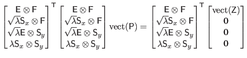
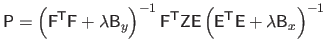
The main advantage of having a data term and a regularization term that can be written using the Kronecker product of matrices is that it leads to efficient computations.
Indeed, given the expressions of the data term and the regularization term, the solution of problem (4.90) is given by:
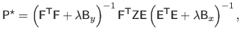 |
(4.97) |
where
 and
and
 .
The solution given by equation (4.99) is derived with the following reasoning:
.
The solution given by equation (4.99) is derived with the following reasoning:
Choice of the Regularization Parameter
At this point, we have an efficient approach to fit a surface to range data (with homoskedastic noise) for a given regularization parameter.
In this section, we propose a new approach to determine in an automatic and fast manner the regularization parameter.
The contribution we propose here is not completely brand new.
In fact, it is an adaptation to our problem of a quite old principle: Morozov's discrepancy principle (130).
In this section, we explain the principles of this criterion in the context of range surface fitting.
Extended details on the Morozov's principle may be found in (141,182,80,168,177).
Again, we emphasize that for now, we just consider a noise with the same distribution over all the dataset.
This stems from the fact that fitting a surface to range data with homoskedastic noise is the basic building block of the whole algorithm that we propose in this section.
The case of the heteroskedastic noise will be handle in section 4.3.2.
Let us consider that the dataset is a noisy sample of a reference function
 , i.e.
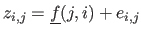 where the
  are random variables that represent the noise.
Let us further assume that the noise has standard deviation
are random variables that represent the noise.
Let us further assume that the noise has standard deviation  .
For a given dataset
.
For a given dataset
 , let
, let
 be the set of all the B-splines control points satisfying equation (4.99) for all possible regularization parameter , i.e. :
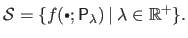 |
(4.98) |
The surface fitting problem is equivalent to find the function
 such that:
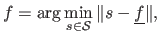 |
(4.99) |
where
 is some kind of function norm.
The discrepancy principle states that the function
is some kind of function norm.
The discrepancy principle states that the function  should be the one that results in a standard deviation for the errors (
 with
with
 ) that is as close as possible to the true one ().
Since
is not necessarily a member of
, the strict equality between and
is not always possible.
The regularization parameter is thus chosen as the one that minimizes the following problem:
) that is as close as possible to the true one ().
Since
is not necessarily a member of
, the strict equality between and
is not always possible.
The regularization parameter is thus chosen as the one that minimizes the following problem:
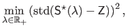 |
(4.100) |
with
 and
and  is the B-spline obtained by solving equation (4.99) for a given value of .
Since the quantity
is the B-spline obtained by solving equation (4.99) for a given value of .
Since the quantity
 increases with , the criterion optimized in equation (4.102) has only one global minimum.
Problem (4.102) may be optimized using, for instance, the golden section search algorithm described in section 2.2.2.12.
increases with , the criterion optimized in equation (4.102) has only one global minimum.
Problem (4.102) may be optimized using, for instance, the golden section search algorithm described in section 2.2.2.12.
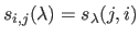
Of course, the ground truth standard deviation of the errors is generally unknown in practice.
In place of that, we propose a simple but efficient approach to estimate the standard deviation of the noise directly from the dataset.
It relies on a local linear approximation of the data.
Let
 be the function representing the plane obtained by linear regression from the dataset
 .
The approximate standard deviation
.
The approximate standard deviation  for all the dataset
is given by:
for all the dataset
is given by:
 |
(4.101) |
The efficiency of this standard deviation estimator for range data will be tested in the experimental part of this section (see section 4.3.3.1).
Note that this estimator is clearly more efficient with data that represent a smooth surface than with data that have discontinuities.
The combination of equation (4.99) and of the discrepancy principle (including the standard deviation estimator) is called the Fast Grid Approach algorithm (FGA).
Note that this algorithm is designed to work on datasets with homoskedastic noise.
It will be used as a basic building block of our more general approach to handle heteroskedastic data.
Our Approach to Handle Heteroskedastic Noise and Discontinuities
In section 4.3.1, we presented the FGA method which allows one to quickly fit a B-spline to range data organized as a regular mesh with homoskedastic noise.
In this section, we present our approach to fit a B-spline on range data with heteroskedastic noise and discontinuities.
The approach we propose to handle such data is a multi-step approach.
The different steps of the algorithm are summarized below and detailed after that.
- Segmentation.
- The dataset is segmented in order to first, separate the different level of noise and second, get rid of the discontinuities.
- Bounding boxes.
- The data of each segment is embedded in a rectangular domain (the bounding box) so that the FGA algorithm can be used.
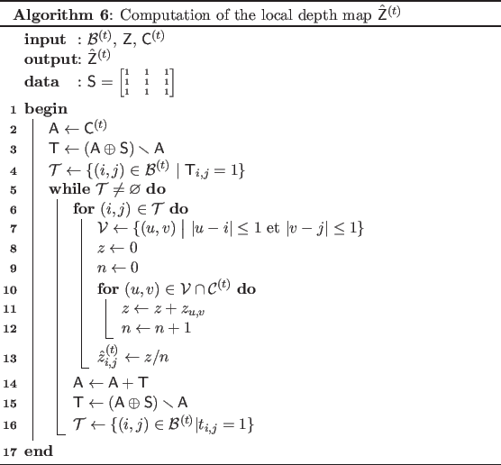
- Local depth maps.
- A local depth map is created for each segment by filling the corresponding bounding box.
- Local fittings.
- A surface is fitted to each one of the local depth maps using the FGA algorithm.
- Merging.
- A single global surface is finally constructed from the local fittings using the fact that the control points of a B-spline have only a localized influence.
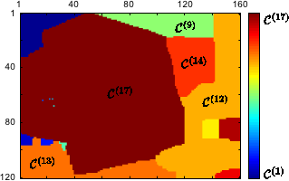
Figure 4.25 illustrates the steps of our approach.
The first step of our approach consists in segmenting the initial dataset according to the depth of the points.
Using this criterion is motivated by the fact that the amount of noise depends mainly on the distance between the sensor and the scene.
Besides, this approach makes the discontinuities coincident with the borders of the segments which is a desirable behaviour in the sense that it is easier to fit a surface on a dataset without discontinuities.
The segmentation is achieved with the  -expansion algorithm of (198,26).
The implementation details are given below.
The result of the segmentation step is a set of
-expansion algorithm of (198,26).
The implementation details are given below.
The result of the segmentation step is a set of  labels
 and a collection of segments
 for
for
 .
The segment
is the set of pixels
.
The segment
is the set of pixels
 labelled with the value
  .
Note that each segment is guaranteed to be 8-connected.
We denote
.
Note that each segment is guaranteed to be 8-connected.
We denote
 the matrix such that
 if
if
 and 0 otherwise.
Let
 be the set of pixels of the depth map
.
The segmentation consists in classifying each pixel of
be the set of pixels of the depth map
.
The segmentation consists in classifying each pixel of
 in one of the segments
 .
Besides, we want the segmentation to be spatially consistent and the segments to be sets of 8-connected pixels.
To do so, we use the -expansion algorithm proposed in (198,26).
With this approach, the segmentation is the solution of an optimization problem:
.
Besides, we want the segmentation to be spatially consistent and the segments to be sets of 8-connected pixels.
To do so, we use the -expansion algorithm proposed in (198,26).
With this approach, the segmentation is the solution of an optimization problem:
 |
(4.102) |
where  is an integer such that
  .
.
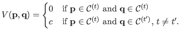
 is the data term, i.e. a term that measures the quality of allocating a certain label to certain pixels.
 is a term promoting the spatial consistency of the segmentation.
We chose as data term the likelihood that a depth belongs to the segment
.
If we consider a normal distribution of parameters
 for the noise in the th segment,
is given by:
for the noise in the th segment,
is given by:
 |
(4.103) |
with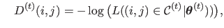 |
(4.104) |
and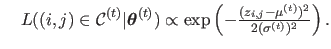 |
(4.105) |
The parameters
 are computed using the k-means algorithm on the depth map
.
The number is determined manually.
The regularization term
is defined using the Potts model (
are computed using the k-means algorithm on the depth map
.
The number is determined manually.
The regularization term
is defined using the Potts model (
 denotes the 8-neighbourhood of the pixel
 ):
):
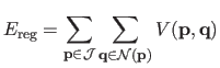 |
(4.106) |
with
The scalar
 determines the weight given to the spatial consistency: we use
  .
The final touch of the segmentation consists in taking the connected components of the segments
.
The final touch of the segmentation consists in taking the connected components of the segments
 .
Usually, the data contained in the segments
.
Usually, the data contained in the segments
 does not form a complete rectangle.
However, the data must be arranged in a full grid so that the FGA algorithm can be used.
To do so, we define for each segment
a bounding box
does not form a complete rectangle.
However, the data must be arranged in a full grid so that the FGA algorithm can be used.
To do so, we define for each segment
a bounding box
 which is, intuitively, a rectangular subdomain of
![$ [k^x_{-k},k^x_{g+k+1}] \times [k^y_{-l},k^y_{h+l+1}]$](img1081.png) that includes the data contained in
and of minimal size.
In other words,
is the smallest rectangular domain
that includes the data contained in
and of minimal size.
In other words,
is the smallest rectangular domain
 (with
(with
 and
and
 ) that contains the non-rectangular domain
 defined as follow:
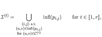 |
(4.107) |
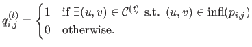
where
 is the domain of influence of the weight
  , i.e. :
![$\displaystyle \mathrm{infl}(p_{i,j}) = [k_j^x,k_{j+k+1}^x] \times [k_i^y,k_{i+l+1}^y].$](img1089.png) |
(4.108) |
Local Depth Maps
Except for some exceptional cases, the data contained in the segment
does not fill completely the bounding box
.
Having a dataset organized as a complete grid is however a requirement to use the FGA algorithm.
We thus define for each segment
a local depth map, denoted
 , which is a rectangular completion of the data contained in
.
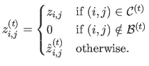
For all
, the local depth map
, which is a rectangular completion of the data contained in
.
For all
, the local depth map
 is defined as:
 |
(4.109) |
The values
 are computed by recursively propagating the depths located on the borders of the class
.
The details of this operation are given by algorithm 6.
Note that the local depth maps
all have the same size than the initial depth map
but they are non-zero only over
.
This makes the merging step easier.
are computed by recursively propagating the depths located on the borders of the class
.
The details of this operation are given by algorithm 6.
Note that the local depth maps
all have the same size than the initial depth map
but they are non-zero only over
.
This makes the merging step easier.
The fourth step of our approach consists in fitting a surface to each one of the depth maps
.
This is achieved using the FGA algorithm of section 4.3.1.
The use of the FGA algorithm is possible because all the requirements are fulfilled: the local depth maps are complete rectangular grids and, moreover, the noise is homogeneous inside each one of the segments.
We use the following parameters for the FGA algorithm:
The result of this step is a collection of matrices of control points
 .
Note that
.
Note that
 if there is no pixel
 such that
 .
The regularization parameter for the th depth map, denoted
.
The regularization parameter for the th depth map, denoted
 , is computed using the data contained in
only, not all the data from
.
The last step of our approach consists in merging all the local fittings in order to get a surface that fits the whole depth map
.
To do so, we build a B-spline by taking the control points computed during the previous step.
For
, let
, is computed using the data contained in
only, not all the data from
.
The last step of our approach consists in merging all the local fittings in order to get a surface that fits the whole depth map
.
To do so, we build a B-spline by taking the control points computed during the previous step.
For
, let
 be the matrix that indicates the control points of `interest' for the segment
, i.e. the ones that have an influence region intersecting with the data contained in
:
be the matrix that indicates the control points of `interest' for the segment
, i.e. the ones that have an influence region intersecting with the data contained in
:
The set of interesting control points is then reduced so that there are no conflicts between the control points coming from different local fittings.
This is achieved by eroding the binary matrix
 :
:
 |
(4.110) |
where
 is the following structuring element:
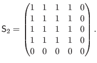 |
(4.111) |
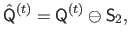
Finally, the surface that fits the whole depth map
is the B-spline having for control points the matrix
 :
:
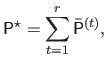 |
(4.112) |
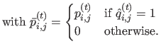 |
(4.113) |
Experiments
Standard Deviation Estimator
In this experiment, we assess the precision of the standard deviation estimator described in section 4.3.1.4.
To do so, we randomly generate some surfaces as linear combination of elementary functions (sine waves, exponential, polynomials).
Depth maps are then obtained by sampling these surfaces on a grid of size
 .
An additive normally-distributed noise with standard deviation is added to the depth maps.
The estimated standard deviation is finally compared to the expected value by computing the relative error between them.
The estimator is tested for several levels of noise ranging from
.
An additive normally-distributed noise with standard deviation is added to the depth maps.
The estimated standard deviation is finally compared to the expected value by computing the relative error between them.
The estimator is tested for several levels of noise ranging from  to
to  of the maximal data amplitude.
The estimation is repeated for 100 surfaces for each level of noise.
We obtain a relative error that is consistently smaller than
of the maximal data amplitude.
The estimation is repeated for 100 surfaces for each level of noise.
We obtain a relative error that is consistently smaller than
 .
.
This experiment shows the interest of exploiting the tensorial properties of the B-spline model instead of the direct approach in order to fit a surface on data arranged as an orthogonal grid.
Figure 4.26 shows the computation times required by the two approaches in function of the number of data points (with slightly less data points than control points).
It is obvious from this illustration that the grid approach is much faster than the direct approach.
We can even say that the grid approach is compulsory if we want to fit surfaces in a reasonable amount of time for large datasets.
Moreover, the memory space required by the direct approach is much more important than for the grid approach.
On our test machine, the computations were intractable for the standard approach with more than 1500 data points.
Figure 4.26:
Illustration of the performance gain obtained when using a grid approach instead of the standard one to fit surfaces on range data.
|
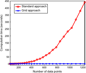 |
Figure 4.27 shows some representative results of our surface fitting algorithm.
These results are compared to the ones obtained with a global regularization scheme.
Since the discrepancy principle is only usable on data with homogeneous noise, we used the generalized cross validation principle (193) to compute the regularization parameter with the global regularization scheme.
It is clear from figure 4.27 that our approach is able to simultaneously use the proper amount of regularization while preserving the sharp edges present in the observed scene.
On the contrary, a global regularization scheme leads to an overly smoothed surface that does not reflect well the scene geometry.
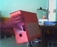
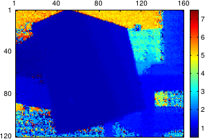
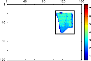
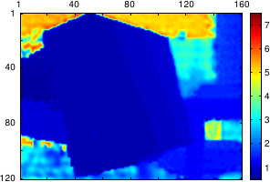
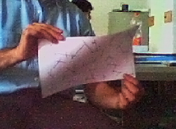
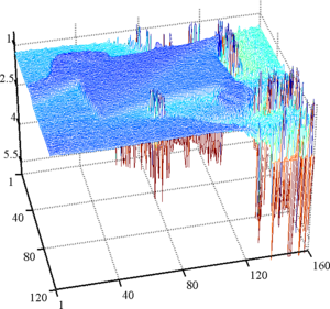
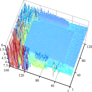
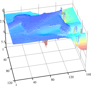
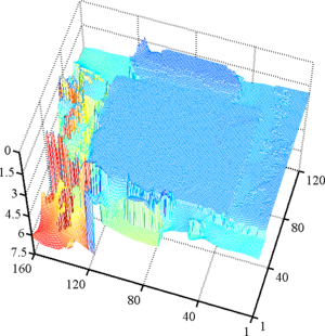
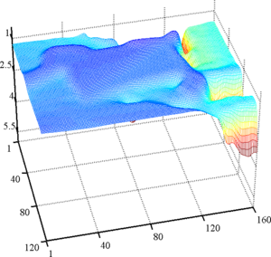
Figure 4.27:
First row: a view of the scene taken with a CMOS sensor. Second row: raw depth maps. Notice the high level of noise present in the background. Third row: surface fitted using our algorithm. Last row: surface fitted using a global approach. With this approach, we can see that the object boundaries are over-smoothed compared to the results obtained with our algorithm.
|
|
In this experiment, we compare the quality of the surfaces fitted using our algorithm described in section 4.3.2 with the ones obtained using a global regularization scheme.
This is achieved by comparing the fitted surface with a ground truth surface.
To do so, we used a set of 214 range images publicly available at (44).
These images were acquired using an Odetics LADAR camera and, as a consequence, the amount of noise is quite limited.
These datasets can thus be used as ground truth surfaces.
Let
 be a range image acquired with the LADAR camera.
The different algorithms are tested using datasets obtained by adding a normally-distributed noise to the LADAR range images with a standard deviation proportional to the depth.
Let
be the noisy dataset:
be a range image acquired with the LADAR camera.
The different algorithms are tested using datasets obtained by adding a normally-distributed noise to the LADAR range images with a standard deviation proportional to the depth.
Let
be the noisy dataset:
 |
(4.114) |
where is a random variable drawn from a normal distribution
 with
with
 .
Let
.
Let  and
and  be the surfaces fitted to the range image
with our algorithm and a global regularization scheme respectively.
Let
be the surfaces fitted to the range image
with our algorithm and a global regularization scheme respectively.
Let
 and
and
 be the depth maps predicted with and respectively.
The quality of the fitted surface is assessed by comparing the norm between the predicted depth maps
and
with the ground truth one
.
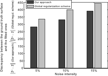
The results, averaged for the 214 range images of the dataset, are reported in figure 4.28 for different levels of noise.
It shows that our approach is, in average,
be the depth maps predicted with and respectively.
The quality of the fitted surface is assessed by comparing the norm between the predicted depth maps
and
with the ground truth one
.
The results, averaged for the 214 range images of the dataset, are reported in figure 4.28 for different levels of noise.
It shows that our approach is, in average,  better than the one using a global regularization scheme whatever the noise intensity is.
Figure 4.28:
Discrepancy between ground truth range images and the ones predicted with the fitted surface using our algorithm (dark grey) and a global regularization scheme (light grey). The indicated level of noise corresponds to the standard deviation of a normally-distributed noise for the deepest point and relative to the total depth of the scene. The surfaces fitted with our approach are better than the ones fitted using a global regularization scheme.
|
 |
Contributions to Parametric Image Registration and 3D Surface Reconstruction (Ph.D. dissertation, November 2010) - Florent Brunet
Webpage generated on July 2011
PDF version (11 Mo)