Subsections
General Points on Image Registration
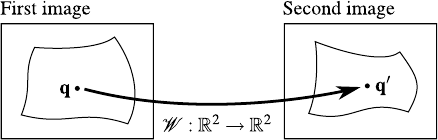
The problem of registering two or more images is to determined a transformation that aligns the input images (101,185).
Note that in thesis, we will mainly consider the case with only two images.
Image registration is a problem that impacts numerous fields such as, to cite a few, computer vision (16,181,205,13), medical imaging (90,204,129,87,203,5,91), or metrology (50,139,78,97).
Broadly speaking, two types of transformation may be estimated (74):
- A geometric transformation that modifies the position of the pixels in the pictures.
- This transformation results in a dense deformation field between a reference image and a target image. Our contributions related to image registration mainly deal with this kind of transformations, especially with non-rigid ones.
- A photometric transformation that modifies the colour of the pixels.
- This transformation models the illumination changes. This type of transformation is not always used when registering two images. This is especially the case when the images are registered using features which are invariant to illumination changes.
Parametric image registration is a classical parameter estimation problem in the sense that, as always, it consists in fixing some parametric model and then determining its parameters from the data by minimizing some criterion.
The parametric model that explains the deformation between the images to register is typically called a warp.
The general principle of image registration is illustrated in figure 5.1.
Figure 5.1:
General principle of image registration. Image registration consists in estimating the transformations that modify an image so that it matches another one. Several type of transformations may be considered. In this thesis, we are mainly interested in geometric transformations.
|
 |
There are two main approaches for parametric image registration: the direct approach and the feature-based approach.
As its name may indicate, the direct approach relies on the information which is directly available such as the colour of the pixels.
With this approach, the criterion to be minimized measures the colour discrepancy between the warped source image and the target image.
In the feature-based approach, the warp parameters are estimated from a finite set of features.
The features are distinctive elements of the images which are first extracted independently in each image to register.
Then, they are matched across the images.
Both approaches have their own advantages and disadvantages.
Other approaches such as cross-validation and frequential approaches may be used to register images.
However, we are not interested in these approaches in this document.
The main advantage of this approach is the high quantity of data used to estimate the warp parameters.
Another good point is that it does not require one to extract and match features.
On the other side, the direct approach is sensitive to changes of appearance.
Besides, it is not suited for registering images with important displacements since the colour information is correlated to the displacement only locally.
Contrarily to the direct approach, the feature-based approach is better suited for large displacements (wide-baseline registration).
Another advantage of the feature-based approach is that they may be robust to illumination changes.
The main drawback of the feature-based approach is that it requires the extraction and the matching of features.
Depending on the nature of the images, there may be only a few feature correspondences which make difficult the estimation of the warp parameters.
This is especially true for badly textured images.
The proportion of false point correspondences (outliers) may also grow quickly when, for instance, the images contains repetitive and undistinguishable patterns.
Once a warp has been estimated between two images, it is natural to deform one of the images in order to align them.
This is something which may be a bit confusing.
Indeed, although the warp is a function from the source image to the target image5.1, it is generally easier to deform the target image.
We call this technique the inverse warping.
It can be achieved without having to compute the inverse warp.
This is realized as follows.
We take an empty picture of the same size than the source image.
The colour of each pixel of this picture (the warped target) is the colour of the corresponding pixel in the target image determined by applying the estimated warp.
With this approach, the target image is not completely warped.
Indeed, the pixels of the target image which do not have an antecedent in the domain of the source image will not be warped.
This can be obviated using the same principle except that we consider an initial domain for the warped target image larger than the one of the source image.
The principle used to warp the target image is illustrated in figure 5.2.
Figure 5.2:
Illustration of the inverse and forward warping.
|
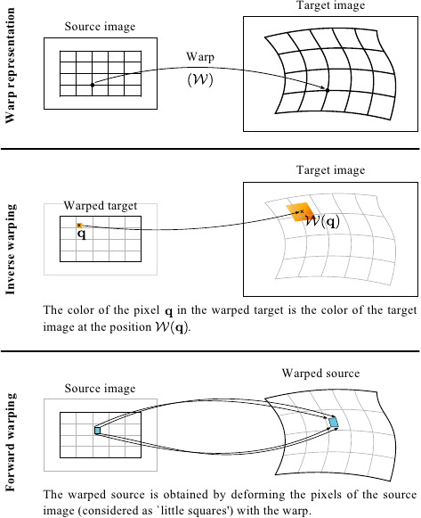 |
If one is ready to make some approximations, it is also possible to make a forward warping of the source image.
Therefore, the source image is aligned to the target image.
This can be achieved by considering the pixels as `little squared area'.
The corners of these squares can then be transformed using the estimated warp.
Even if we use deformable warps, the pixels are transformed in a rigid way.
Practically, the warped source image can be represented as a vectorial image.
It can then be converted to a bitmap using a standard graphical library such as Cairo5.2.
Although quite natural, this approach has the major drawback of being much heavier in terms of computational time than the inverse warping.
The forward warping is illustrated in figure 5.2.
As it will become clearer later in this chapter, most of the approaches to image registrations requires one to compute the derivatives of images.
Indeed, since image registration is formulated as an optimization problem, the optimization algorithms often need derivative information such as the gradient or the Hessian matrix.
Let
 be an image.
It is a common assumption to consider that
is defined over a rectangular bounded subdomain of
be an image.
It is a common assumption to consider that
is defined over a rectangular bounded subdomain of
 .
However, in practice, this is not quite true.
Indeed, a digital image is defined over a rectangular bounded subdomain of
.
However, in practice, this is not quite true.
Indeed, a digital image is defined over a rectangular bounded subdomain of
 .
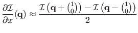
Therefore, one of the most simple technique to compute the derivatives of an image consists in using finite differences.
Finite differences come in different flavours.
For instance, if we consider the derivative of the image
with respect to
.
Therefore, one of the most simple technique to compute the derivatives of an image consists in using finite differences.
Finite differences come in different flavours.
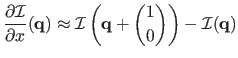
For instance, if we consider the derivative of the image
with respect to  , i.e. the first free variable of the function, then we have:
- Forward finite differences:
 |
(5.1) |
- Backward finite differences:
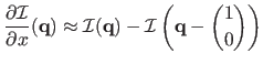 |
(5.2) |
- Central finite differences:
 |
(5.3) |
In this document, the default choice is the forward finite differences.
Note that there exists other more complex techniques to evaluate the derivatives of a discrete function (see, for instance, (119,30).
Image Registration as an Optimization Problem
Image registration may be cast into a parameter estimation problem.
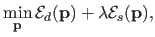
In its most generic form, the non-rigid image registration problem is written as:
 |
(5.4) |
where
 is the vector containing the parameters of the warp (such as the control points of a B-spline).
 is the data term which compares the information between the source and the target images.
The term
is the data term which compares the information between the source and the target images.
The term
 is the smoothing term that regularizes the warp.
The hyperparameter
is the smoothing term that regularizes the warp.
The hyperparameter  controls the relative importance of the data and smoothing terms.
We now give some details of the different terms presented in equation (5.4).
controls the relative importance of the data and smoothing terms.
We now give some details of the different terms presented in equation (5.4).
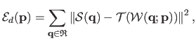
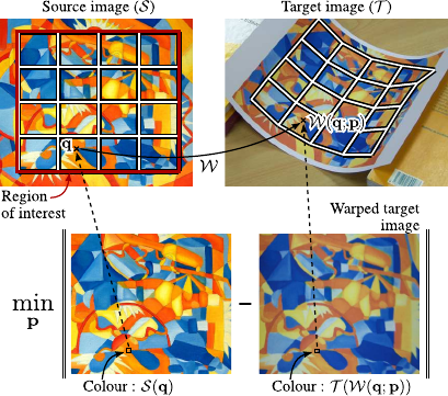
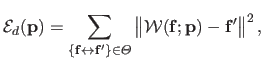
The most common data term for the direct approach to image registration is the sum of squared difference (SSD).
It is computed between the source image and the target image deformed with the estimated warp:
 |
(5.5) |
where
 is the region of interest (ROI).
It is a set of pixels of the source image that should be carefully chosen.
More details on this region of interest along with some of our contributions related to this matter will be given in section 5.2.
The principle of the SSD term for direct image registration is illustrated in figure 5.3.
is the region of interest (ROI).
It is a set of pixels of the source image that should be carefully chosen.
More details on this region of interest along with some of our contributions related to this matter will be given in section 5.2.
The principle of the SSD term for direct image registration is illustrated in figure 5.3.
Figure 5.3:
Illustration of the principle of the SSD term for direct image registration. The SSD term is the sum of the difference of colours of the pixels in the ROI (in the source image) and their correspondent in the target image (computed using the warp induced by the parameters  ).
).
|
 |
The Mutual Information (MI) is another common principle to image registration that raises a different data term.
It has been independently introduced in (48,192).
Note that we do not use this kind of criterion in the rest of this document.
The MI is the quantity of information of the first image which is contained in the second image.
The MI is maximal when the two images are identical.
There exists several definitions.
We report here the resulting data term presented in (74):
 |
(5.6) |
where  is the Shannon entropy (173).
It measures the quantity of information contained in a sequence of events.
The entropy of an image is related to its complexity.
A completely untextured image has a low entropy while a highly textured image has a higher value.
The joint entropy
is the Shannon entropy (173).
It measures the quantity of information contained in a sequence of events.
The entropy of an image is related to its complexity.
A completely untextured image has a low entropy while a highly textured image has a higher value.
The joint entropy
 measures the quantity of information shared by the images
 and
and
 .
If these images are identical then their joint entropy is minimal.
It may be computed from the joint histogram of the two images.
Maximizing the MI is thus equivalent to searching for the transformation that results in a maximum of information in the images while having the images as similar as possible.
Contrarily to the other types of approaches, the MI criterion does not rely directly on the colour information.
It makes the MI criterion particularly well-suited for multi-modal image registration.
This is the reason why the MI criterion is very popular in medical image registration (129,150,162).
.
If these images are identical then their joint entropy is minimal.
It may be computed from the joint histogram of the two images.
Maximizing the MI is thus equivalent to searching for the transformation that results in a maximum of information in the images while having the images as similar as possible.
Contrarily to the other types of approaches, the MI criterion does not rely directly on the colour information.
It makes the MI criterion particularly well-suited for multi-modal image registration.
This is the reason why the MI criterion is very popular in medical image registration (129,150,162).
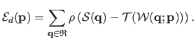
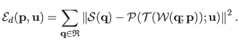
Typically, the data term used in feature-based image registration measures the (squared) Euclidean distance between the features of the source image transformed with the warp and the features of the target image.
This may be written as:
 |
(5.7) |
where  is a set of feature correspondences that was previously detected and matched in the images.
A simple yet powerful extension of the above-mentioned data term consists in using an M-estimator instead of a squared Euclidean distance.
This allows one to get estimation procedures more robust to erroneous data.
Erroneous data are very common and almost unavoidable with the two most common approaches to image registration.
For instance, in the feature-base approach, the are often false feature correspondences.
This generally comes from a poor extraction of the features or from a bad matching of the features.
The standard non-robust data term for feature-based image registration is modified with an M-estimator in the following way:
 |
(5.8) |
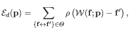
In the case of the direct approach, outliers are due to phenomena such as occlusions and specularities.
Indeed, if such phenomena arise then the colour of two corresponding pixels may be quite different.
The use of an M-estimator in the direct approach has been utilized in, for instance, (7,137).
With an M-estimator, the initial data term of the direct approach is transformed into the following one:
 |
(5.9) |
As we said in equation (5.4), the cost function for non-rigid image registration generally includes a smoothing term (also known as regularization term).
Many such terms have been proposed in the literature.
For instance, one may use the smoothing term of order 1 proposed in (98):
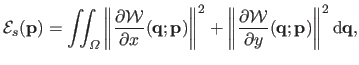 |
(5.10) |
where  is the definition domain of the warp
 .
Alternatively, one may use a smoothing term of second order : the bending energy.
It is similar to the bending energy used in the previous chapter for range data fitting.
With a warp, which is a function from
to
, the bending energy is defined by:
.
Alternatively, one may use a smoothing term of second order : the bending energy.
It is similar to the bending energy used in the previous chapter for range data fitting.
With a warp, which is a function from
to
, the bending energy is defined by:
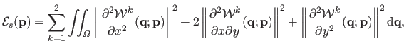 |
(5.11) |
where
 and
and
 are respectively the first and the second coordinates of
.
are respectively the first and the second coordinates of
.
Here, we present some more advanced topics on the direct methods for image registration.
We keep talking about general elements.
The basic criterion of equation (5.5) for the direct approach to image registration is extremely sensitive to illumination changes.
Indeed, there may be some important discrepancies in the colour of the corresponding pixels between images taken under different circumstances (lighting conditions, cameras, etc.)
There exists several approaches to obviate this problem.
For instance, the illumination changes can be explicitly modelled by adding a photometric transformation in the criterion.
The criterion thus becomes:
 |
(5.12) |
The transformation
 parametrized by the vector
 represents the illumination changes.
Therefore, the optimization takes place simultaneously over
and
.
This type of approach has been used in, for instance, (178,11).
represents the illumination changes.
Therefore, the optimization takes place simultaneously over
and
.
This type of approach has been used in, for instance, (178,11).
Another solution to overcome the problems related to illumination changes is to estimate the geometric transformation on data invariant to such changes.
For instance, a normalization of the images may introduce some kind of robustness to global illumination changes (such global transformation might appear when the images to register have been taken with different cameras).
In (148), the images are converted into a different colour space which is invariant to shadows.
One major drawback of the direct approaches to image registration is the fact that they are usually able to estimate the deformation only if it is not too wide.
A partial remedy to this problem is the use of a multi-scale approach (112).
The underlying idea of such approaches is to first estimate the geometric deformation on a low resolution version of the images and then propagating the estimated deformation to higher resolutions.
A pyramid of images is thus constructed along with the registration process.
Several techniques may be used to construct a low resolution version of an image.
For instance, one may compute the value of a pixel at the level  as a weighted mean of the pixels at the level
  .
The weights are typically determined with a bell-shaped Gaussian curve.
Note that in image registration, the multi-scale approach works quite well for large translations.
For other types of geometric transformation, it is generally less efficient.
.
The weights are typically determined with a bell-shaped Gaussian curve.
Note that in image registration, the multi-scale approach works quite well for large translations.
For other types of geometric transformation, it is generally less efficient.
We now give some supplementary details on the feature-based approach to image registration.
In particular, we quickly review some very common types of features.
We also say a word on the important step of matching the features.
Detecting and matching feature is the first step in feature-based image registration, nonetheless essential to successfully register images.
Features are distinctive elements of an image.
They can be viewed as a high level representation of an image since they abstract the content of an image.
There exists many types of features.
In a nutshell, features can be classified into two main categories : the point-wise features (keypoints) and the area-based one.
An algorithm in charge of extracting features is named a detector.
In addition to a spatial information, a descriptor is often associated to a descriptor.
The descriptor can be viewed as a characteristic signature of the feature.
They are used to couple the features across several images relying on the principle that features with similar descriptors are likely to represent the same point.
A desirable property for any feature is to be invariant, i.e. to have a descriptor that does not depend too much on certain transformations.
For instance, a feature can be invariant to a change of illumination or to a geometric transformation such as a rotation.
We now give some explanations on the most commonly used features in image registration.
Supplementary general informations on features may be found in, for instance, (181,188).
SIFT (Scale Invariant Feature Transform) is one of the most popular keypoint detectors.
It has been introduced in (114).
The SIFT feature descriptors are invariant to scale, orientation, and partially invariant to illumination changes (115).
It has also been shown to perform quite well under non-rigid deformations (63).
We now give the general idea behind the SIFT detector.
We do not give here the detailed algorithm since it is not the core of this work.
In the rest of this document, features detectors are just tools we sometimes use in experiments.
With SIFT, the locations of the keypoints are the minima and the maxima of the result of Difference Of Gaussians applied to a pyramid of images built from the initial image by smoothing and resampling.
Using a pyramid of images makes SIFT invariant to the scale.
The points obtained in this way are then filtered: points with low contrast and points along edges are discarded.
The dominant orientations of the resulting keypoints are then computed.
The description of the keypoints are computed relatively to the dominant orientations.
This allows one to be invariant to the orientation.
The SIFT descriptor (typically a sequence of 128 bytes) is finally computed by considering the pixels around a radius of the keypoint location.
This descriptor encodes an orientation histogram computed for all the pixels in the neighbourhood of the keypoint.
SURF (Speeded Up Robust Features) is another keypoint detector which shares many similarities with SIFT.
It was first introduced in (19).
Supplementary details may be found in (20).
The main advantage of SURF is that it is much faster than SIFT.
SURF is built on the same concepts than SIFT but with some radical approximations to speed up the detection process (172).
Instead of using a the difference of Gaussian operator to detect the maxima and the minima in the pyramid of images, SURF uses the determinant of the Hessian.
The descriptor associated to the keypoints are also similar to the one produced by SIFT.
It is computed from orientation histograms in a square neighbourhood centred at the keypoint location.
The resulting descriptor is a vector of 64 elements.
MSER (Maximally Stable Extremal Region) is one of the most common method to detect area-based regions in images.
It was developed by (122) to find correspondences between image areas from two images with different points of views.
Additional information may be found in (188,127,128).
It relies on the concept of extremal region.
Let
be an image and let  be a contiguous region of
.
Let us denote
be a contiguous region of
.
Let us denote
 the contour of the region .
is an extremal region if either
the contour of the region .
is an extremal region if either
 (maximum intensity region) or
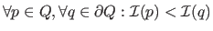 (minimum intensity region).
A maximally stable extremal region is defined as follows.
Let
(minimum intensity region).
A maximally stable extremal region is defined as follows.
Let
 be a sequence of nested extremal regions.
The region
be a sequence of nested extremal regions.
The region
 is maximally stable if and only if the quantity
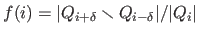 has a local minimum at
  .
.
 is a parameter of the method.
MSER has many interesting properties.
For instance, it is invariant to affine transformation of image intensities.
It is also stable: only the regions whose support is nearly the same over a range of thresholds are selected.
MSER automatically detects regions at different scales without having to explicitly build an image pyramid.
Computing the MSER regions can be achieved quite rapidly (135).
Besides, MSER has been compared to other region detectors in (128) and it has been shown to consistently give the best results for many tests.
MSER is therefore a reliable region detector.
Contributions to Parametric Image Registration and 3D Surface Reconstruction (Ph.D. dissertation, November 2010) - Florent Brunet
Webpage generated on July 2011
PDF version (11 Mo)