Subsections
Direct Image Registration without Region of Interest
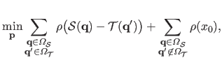
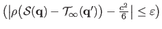
As a reminder of section 5.1.2.1, direct image registration in its most basic form amounts to solve the following minimization problem:
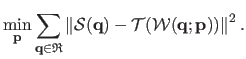 |
(5.13) |
For the sake of simplicity, we forget about the regularization term in equation (5.13) since it is not of central importance in the contribution proposed in this section.
We also remind here the classical variant of equation (5.13) which consists to use an M-estimator in order to get a robust registration algorithm:
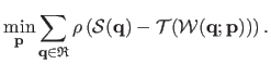 |
(5.14) |
This formulation is important in this section since the proposed contribution relies on it.
In this section, we present a contribution we made concerning direct image registration.
More precisely, this contribution deals with the problems related to the region of interest (ROI).
As it will be explained later in this section, the ROI may represent a major difficulty when doing direct image registration.
Here, we propose a new solution that allows one to use the direct approach to register images without needing a ROI.
This is made possible by a wise use of the robust framework to direct image registration that relies on saturated M-estimators.
As said previously in this chapter, standard direct image registration consists in estimating the geometric warp between a source and a target images by maximizing the photometric similarity for the pixels of a Region of Interest (ROI).
The ROI must be included in the real overlap between the images otherwise standard registration algorithms fail.
As it will be shown later, determining a proper ROI is a hard `chicken-and-egg' problem since the overlap is only known after a successful registration.
Almost all algorithms in the literature consider that the ROI is given.
This is generally either inconvenient or unreliable.
In this section we propose a new method that registers two images without using a ROI.
The key idea of our method is to consider the off-target pixels as outliers.
We define the off-target pixels as those pixels of the source image mapped outside the target image by the current warp.
We use the classical robust M-estimation framework to handle both the off-target pixels and the usual outliers caused, for instance, by occlusions.
With our formulation, the true image overlap is defined as the set of inliers.
Experiments on synthetic and real data with the homography and Free-Form Deformation based on B-splines show that our method outperforms standard approaches in terms of accuracy and robustness while precisely retrieving the overlap in the source and target images.
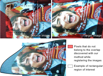
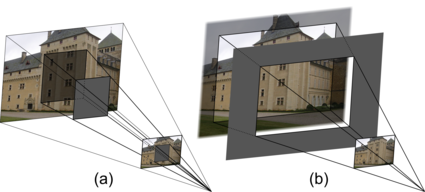
Figure 5.4:
We propose a new algorithm that does not require one to define a region of interest (ROI). Our algorithm discovers the exact overlap between two images while registering them.
Using the rectangular ROI in dashed line defeats classical methods since it contains pixels that do not belong to the overlap.
|
 |
The direct approach to image registration is interesting because it does not rely on feature correspondences.
However, standard registration algorithms require a ROI
 included in the overlap of the images.
This is a difficult `chicken-and-egg' problem since the overlap can only be determined after a successful registration.
There is no known satisfactory solution to this problem.
included in the overlap of the images.
This is a difficult `chicken-and-egg' problem since the overlap can only be determined after a successful registration.
There is no known satisfactory solution to this problem.
Let
 be the image overlap, i.e. the set of pixels of the source image that are also seen in the target image:
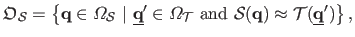 |
(5.15) |
where
 is the pixel
 transformed with the true deformation between
 and
and
 .
It is obvious that the cost function equation (5.13) or equation (5.14) cannot be evaluated at those pixels that do not belong to
.
As a consequence,
must be included in
, otherwise the registration algorithms based on equation (5.13) or equation (5.14) will fail.
Besides, it is better to have a ROI as large as possible in order to have the greatest quantity of information to estimate the warp.
The problem here is that the real overlap
is known only after a successful registration of the images.
.
It is obvious that the cost function equation (5.13) or equation (5.14) cannot be evaluated at those pixels that do not belong to
.
As a consequence,
must be included in
, otherwise the registration algorithms based on equation (5.13) or equation (5.14) will fail.
Besides, it is better to have a ROI as large as possible in order to have the greatest quantity of information to estimate the warp.
The problem here is that the real overlap
is known only after a successful registration of the images.
As we will review in section 5.2.2.1, the ROI is often a polygonal region in the source image defined either by the user or by some ad hoc means (11).
This lacks automatism and may be unreliable.
The adaptive ROI (147) is another approach.
It considers the entire domain of the source image as an initial ROI and updates it during the optimization process.
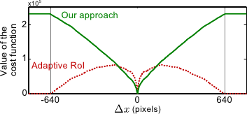
As we will review in section 5.2.2.2, the cost function of (147) is extremely hard to minimize and has global minima that do not correspond to the correct solution (see figure 5.5).
We propose a novel approach to direct image registration.
It is fundamentally different from standard approaches in that it does not need a ROI.
This is made possible by considering the off-target pixels as outliers;
the theoretical foundations of this principle are explained in section 5.2.3.
The cost function we propose to optimize takes into account all the pixels of the source image.
A fixed penalty that corresponds to the one given to usual outliers is associated to the off-target pixels.
We then use the standard robust M-estimation framework of equation (5.14) to handle both the usual outliers and the off-target pixels in a unified way.
Our new approach has several advantages.
First, the proposed cost function does not have trivial minima (see figure 5.5).
Second, it solves all the above-mentioned problems related to the ROI.
Third, the overlap is automatically obtained as the set of inliers.
Rectangular Region of Interest
A common approach used to define the ROI consists in guessing a maximal per-pixel displacement.
The ROI is then chosen as a rectangle obtained by removing to the source image domain a margin of width larger than the hypothesized maximal displacement.
Ideally, the width of this margin should be as close as possible to the actual maximal displacement, rarely known before registration.
The margin width is commonly overestimated so that the optimization algorithm will not fail.
Nonetheless, a large ROI provides more information to estimate the warp accurately.
Moreover, the size of the ROI affects the profile of the cost function in equation (5.5).
A simple experiment inspired by (147) illustrates this phenomenon.
Figure 5.6 shows, for different margin sizes, the evolution of the cost function versus a single shift parameter  (the amplitude of a translation along the
  -axis).
The source and the target images are identical except for a Gaussian noise with standard deviation equal to
-axis).
The source and the target images are identical except for a Gaussian noise with standard deviation equal to  of the maximal pixel value.
Figure 5.6 shows that a small margin (a large ROI) results in a smooth cost function but has dramatically restricted range of admissible translations.
Using a larger margin (a smaller ROI) increases the range of possible translations but creates a lots of local minima in the cost function.
of the maximal pixel value.
Figure 5.6 shows that a small margin (a large ROI) results in a smooth cost function but has dramatically restricted range of admissible translations.
Using a larger margin (a smaller ROI) increases the range of possible translations but creates a lots of local minima in the cost function.
Figure 5.6:
Profile of the data term of equation (5.5) for rectangular ROI with margins ranging from 10 to 130 pixels (for images of size
 ).
).
|
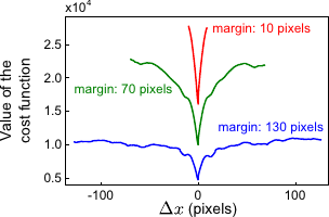 |
Table 5.1:
Respective advantages and disadvantages of the large and small margins. Note that neither of them has all the advantages.
|
| |
Large margin (small ROI) |
Small margin (large ROI) |
| Range of admissible transformations |
+ |
- |
| Quantity of information available for the registration |
- |
+ |
|
Adaptive Region of Interest
An alternative to the rectangular ROI has been proposed in (147).
In this approach, the fixed ROI
is replaced by an adaptive ROI
 .
The minimization problem thus becomes:
.
The minimization problem thus becomes:
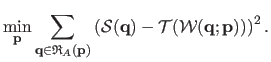 |
(5.16) |
For a given set of parameters
 ,
contains all the pixels (except for a 1-pixel margin used to compute the target image derivatives by finite differences) from the source image that, once warped, belongs to the domain of the target image, i.e.
,
contains all the pixels (except for a 1-pixel margin used to compute the target image derivatives by finite differences) from the source image that, once warped, belongs to the domain of the target image, i.e.
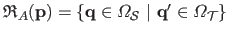 with
with
 .
Although this method does not require one to define a ROI, it is not fully satisfactory.
First, problem (5.16) is badly posed in the sense that there exists an infinite number of minima that do not correspond to the correct warp parameters.
These minima appear when there is no overlap between the source and the warped target images.
This fact is illustrated with an experiment similar to the one used in section 5.2.2.1.
We observe in figure 5.5 that the cost function of problem (5.16) is null (and thus minimal) as soon as the domains do not overlap (
.
Although this method does not require one to define a ROI, it is not fully satisfactory.
First, problem (5.16) is badly posed in the sense that there exists an infinite number of minima that do not correspond to the correct warp parameters.
These minima appear when there is no overlap between the source and the warped target images.
This fact is illustrated with an experiment similar to the one used in section 5.2.2.1.
We observe in figure 5.5 that the cost function of problem (5.16) is null (and thus minimal) as soon as the domains do not overlap (
 ).
Second, the fact that
depends on
makes problem (5.16) hard to solve rigorously.
The authors of (147) propose to neglect the dependency on
and alternate the estimation of
).
Second, the fact that
depends on
makes problem (5.16) hard to solve rigorously.
The authors of (147) propose to neglect the dependency on
and alternate the estimation of
 and
.
Third, the adaptive ROI algorithm is not robust to outliers and, as such, it cannot properly handle occlusions and specularities.
and
.
Third, the adaptive ROI algorithm is not robust to outliers and, as such, it cannot properly handle occlusions and specularities.
Direct Image Registration without Region of Interest
We propose a new method to direct image registration that does not need a ROI.
It thus avoids the above mentioned problems related to the ROI.
Our new cost function uses all the pixels of the source image, as the adaptive ROI of (147).
However, as the example of figure 5.6 shows, our cost function has no trivial minima.
We will show that it is also much easier to optimize rigorously.
The key idea of our method is to penalize the off-target pixels with a fixed cost.
The cost associated to the other pixels remains the usual robust colour discrepancy of equation (5.14).
To some extent, this maximizes the size of the overlap between the two images.
We use the same penalty for the off-target pixels and the outlying pixels, for reasons explained below.
Figure 5.7:
Pixels out of the field of view (b) can be considered as usual outliers (a).
|
 |
Imagine a target camera with an unbounded field of view.
Such a camera would produce images with an infinite domain.
Imagine now that a plane with a rectangular hole is placed between the camera and the observed scene, as figure 5.7 (b) illustrates.
The part of the scene visible through the hole corresponds to the actual target image
.
The rest of the scene is not seen because it is occluded by the plane, exactly as for the pixels hidden by an external occluder, as shown in figure 5.7 (a).
With this reasoning, it becomes natural for one to handle off-target pixels as usual outliers.
A direct yet incomplete mathematical statement of our idea is the following minimization problem:
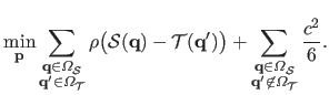 |
(5.17) |
Here, we consider that the M-estimator is the Tukey's M-estimator, detailed in section 3.1.2.2.
As a reminder, the  -function of this M-estimator is:
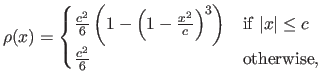 |
(5.18) |
where  is a constant tuning the sensitivity of the M-estimator to outliers.
We use this particular M-estimator because it has the interesting property of being saturated, i.e. it is constant after a certain threshold ().
Note that the second term in equation (5.17) corresponds to the value given to outliers by the Tukey's M-estimator.
Solving problem (5.17) is difficult since two sums are mixed, with a number of terms varying as a function of
since
.
First of all, we rewrite the fixed penalty term:
is a constant tuning the sensitivity of the M-estimator to outliers.
We use this particular M-estimator because it has the interesting property of being saturated, i.e. it is constant after a certain threshold ().
Note that the second term in equation (5.17) corresponds to the value given to outliers by the Tukey's M-estimator.
Solving problem (5.17) is difficult since two sums are mixed, with a number of terms varying as a function of
since
.
First of all, we rewrite the fixed penalty term:
 |
(5.19) |
where  is any value saturating the M-estimator:
 .
With the bisquare -function, any value such that
.
With the bisquare -function, any value such that
 is suitable (see equation (5.18)).
Problem (5.19) can be rewritten:
is suitable (see equation (5.18)).
Problem (5.19) can be rewritten:
![$\displaystyle \min_{\mathbf{p}} \sum_{\mathbf{q} \in \Omega_{\mathcal {S}}} \rh...
... {T}(\mathbf{q}')\big) + [\mathbf{q}' \not\in \Omega_{\mathcal {T}}] x_0 \Big),$](img1186.png) |
(5.20) |
where ![$ [ ]$](img1187.png) is the operator such that
is the operator such that ![$ [a]=1$](img1188.png) if
if  is true and
 ![$ [a] = 0$](img1189.png) otherwise.
We rewrite problem (5.20) by introducing the image
otherwise.
We rewrite problem (5.20) by introducing the image
 :
:
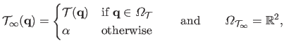 |
(5.21) |
where  is any value such that
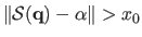 .
Finally, our method is to solve:
.
Finally, our method is to solve:
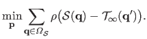 |
(5.22) |
Problem (5.22) is solved with standard Iteratively Reweighed Least-Squares (see section 2.2.2.11) or with a more generic algorithm such as Newton's method (see section 2.2.2.4).
An interesting property of our approach is that it automatically discovers the overlap.
For instance, with Tukey's bisquare M-estimator, a pixel
such that
 can be considered as an outlier (with
 a small constant, e.g.
  ).
The overlap in the source image is the set of source pixels satisfying this condition.
The overlap in the target image is the warped source overlap.
Recovered overlaps are illustrated in figure 5.4 and in section 5.2.4.2.
).
The overlap in the source image is the set of source pixels satisfying this condition.
The overlap in the target image is the warped source overlap.
Recovered overlaps are illustrated in figure 5.4 and in section 5.2.4.2.
Experimental Results
Synthetic Data
We generated synthetic data in the following manner.
First, a warp (homography or B-spline) is determined by interpolating some randomly generated point correspondences.
The source image is obtained by unravelling a texture image with the previously computed warp and the texture image is used as the target image.
The average distance between the point correspondences controls the warp magnitude  (in pixels).
A proportion of the source and target images is then replaced with data from a different image to simulate occlusions.
Last, Gaussian noise with standard deviation
(in pixels).
A proportion of the source and target images is then replaced with data from a different image to simulate occlusions.
Last, Gaussian noise with standard deviation  is added to the images.
We used colour images with intensities coded with real values between 0 and 1.
The images are
is added to the images.
We used colour images with intensities coded with real values between 0 and 1.
The images are
 pixels wide.
Figure 5.8 gives an illustration of the generation process.
pixels wide.
Figure 5.8 gives an illustration of the generation process.
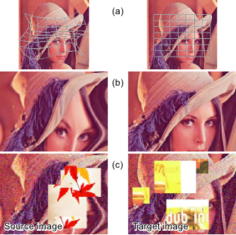
Figure 5.8:
Synthetic data generation. (a) Texture image and deformation used to generate the source and the target images. (b) The warp is unravelled to generate the source image. (c) Noise and outliers are added to the images.
|
 |
The influence of several factors is studied: the transformation magnitude , the amount of noise and the proportion of erroneous data .
Each one of these factors is studied independently with default values:
 pixels,
 and
and
 (10% of the maximal pixel intensity value).
Several algorithms are compared: rectangular ROI (RECT), the adaptive ROI of (147) (ADAP) and our approach (MAXC).
Different variants of the RECT algorithm are considered: narrow (10%) and large (25%) margins without M-estimator (RECTN, RECTL) and with M-estimator (RECTNM, RECTLM).
The reported results are averages over 100 trials.
(10% of the maximal pixel intensity value).
Several algorithms are compared: rectangular ROI (RECT), the adaptive ROI of (147) (ADAP) and our approach (MAXC).
Different variants of the RECT algorithm are considered: narrow (10%) and large (25%) margins without M-estimator (RECTN, RECTL) and with M-estimator (RECTNM, RECTLM).
The reported results are averages over 100 trials.
As explained in section 5.2.2.1, a ROI of fixed size can lead to a failure of the optimization process.
Figure 5.9 shows in which proportion such failures occur for the experiments of the next 3 paragraphs and for the default values.
Note that convergence towards a false solution (local minimum) is not counted as a failure.
We observe that there are more failures with a wide rectangular ROI (RECTN) than with a small one (RECTL).
There are less failures with an M-estimator (RECTNM, RECTLM) than without because the steps of the optimization algorithms tend to be smaller.
In the sequel, when an algorithm fails to converge, the reported measurements are from the last valid iteration.
Figure 5.9:
Failure rates. ADAP and MAXC never fail because they do not rely on a fixed ROI.
|
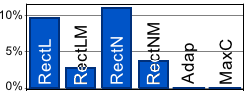 |
Figure 5.10 shows the number of iterations.
Overall, the convergence is faster with the homographic than with the B-spline warp.
This comes from the fact that the homographic warp is global.
The apparent rapidity of the algorithms relying on a rectangular ROI stems from the fact that these algorithms can fail before convergence when the given ROI is not valid.
Our approach, MAXC is generally better than ADAP which is the only other method that does not require a ROI.
However, MAXC takes more iterations to converge when the transformation magnitude is large.
This is explained by the fact that many pixels from the source image, once transformed, do not belong to the target image domain.
The convergence is slightly slowed down since these pixels are penalized with our approach.
Figure 5.10:
Influence of several factors on the the number of iterations. The number of iterations done by the algorithms based on a rectangular ROI is relatively low because these methods can stop prematurely (fail) as soon as the ROI is not valid.
|
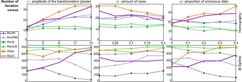 |
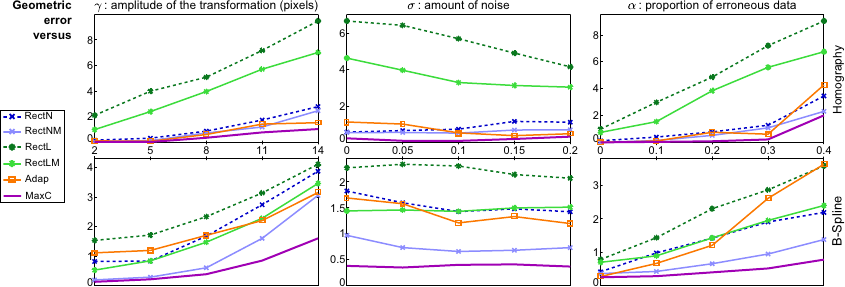
Figure 5.11 shows the geometric error, the discrepancy in pixels between the estimated and the ground truth transformations.
We observe that the amount of noise does not influence much the performance of the algorithms.
On the contrary, the geometric error is influenced by the transformation magnitude and by the proportion of outliers.
This is especially true for the approaches that do not include an M-estimator.
Compared to the other methods, our approach is the one that gives the best results.
We can see that, with our approach, the geometric error is often less than one pixel.
This result is particularly important because it shows that our approach is not biased by the penalty term used for the pixels which are warped outside of the target domain.
Figure 5.11:
Influence of several factors on the geometric error. Our approach (MAXC) gives the best results. Globally, the approaches relying on M-estimators are the best ones.
|
 |
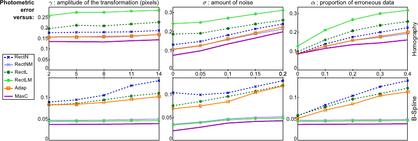
The average photometric error obtained after the last iteration of the studied algorithms is reported in Figure 5.12.
The smallest errors are always obtained with our approach whatever the varying factor and the geometric transformation are.
Figure 5.12:
Influence of several factors on the photometric error. The best results are always obtained with our approach whatever the transformation model and whatever the studied factor.
|
 |
Real Data
We consider a source and a target images of a planar scene taken from two different view points and with an occlusion in the target image.
Under these conditions, the warp between the two images is a homography. Figure 5.13 shows the ROI used during the last iteration of four different algorithms.
This ROI is shown in both the source and the target images.
The difference image between the warped target and the source images is also shown.
It shows that our approach, MAXC, is the only one to estimate the correct homography.
The main point of figure 5.13 is that the final ROI determined with MAXC corresponds exactly to the true overlap between the images.
The ROI used by ADAP at convergence does not take into account the occluder.
Consequently, ADAP is not able to recover correctly the homography.
The ROI utilized by RECTLM does not contain enough pixels making this approach unable to determine precisely the homography.
Finally, the algorithm RECTNM fails to converge since its ROI contains pixels that do not belong to the overlap (figure 5.13 shows the last valid iteration).
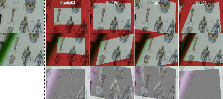
Figure 5.13:
Examples of registration results for different algorithms.
The first row corresponds to the source image, the second row to the target image, and the last row to the difference between the source and the warped target image. The red pixels are the pixels not included in the ROI during the last iteration of the algorithms.
Note that the ROI computed by our approach (MAXC) corresponds to the true overlap (taking into account both the field of view and the occluder). Our approach is the only one that successfully registers this pair of images.
|
 |
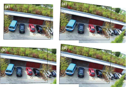
We consider a video captured by a camera that rotates around its optical centre with a uniform movement from left to right.
Consequently, the successive images are linked with homographies.
The goal of this experiment is to build a panorama as wide as possible by taking the first image of the video and the furthest image for which the registration is successful.
As shown in figure 5.14, the widest panoramas are obtained with ADAP and MAXC.
For this video, there are no occluders and, thus, the results of ADAP and MAXC are similar.
The algorithms RECTN and RECTL get the smallest panoramas since the maximal displacements are dictated by margin sizes.
Figure 5.14:
Panorama calculated with (a) RECTN, (b) RECTL, (c) ADAP and (d) MAXC. The widest panoramas are obtained with ADAP and our approach: MAXC.
|
|
An example of deformable registration using our method is given in figure 5.15.
This figure illustrates that our approach automatically retrieves the true overlap in both the source and the target images.
Note that a video corresponding to that example is provided as supplemental material.
Figure 5.15:
Example of deformable mosaic. (a): source image ; (b): target image ; (c) mosaic. The red pixels in (a) and (b) are the pixels that do not belong to the overlap determined with our approach.
|
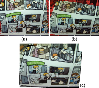 |
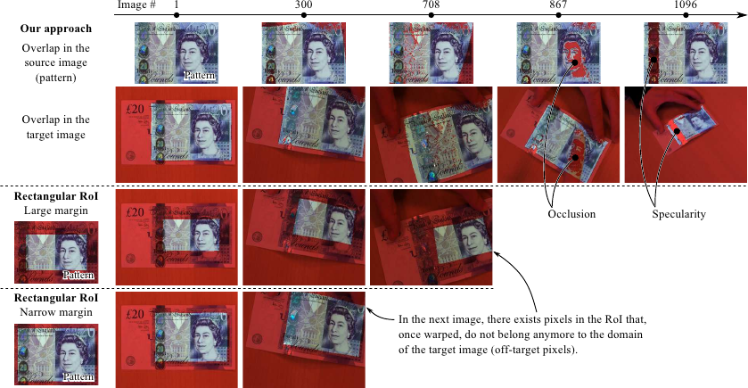
Figure 5.16 illustrates the tracking of a pattern in a video sequence.
Three approaches are compared: our approach, and two approaches using a fixed rectangular ROI (defined with either a large margin or a narrow margin).
The object to track is a deforming banknote.
We thus use a FFD warp with
 control points.
The pattern (i.e. the source image) to track is defined as a part of the first image in the video sequence.
The pattern is registered in each new image (which plays the role of the target image) using as an initial solution the registration determined for the previous image.
Figure 5.16 shows that the approaches relying on fixed ROI fail as soon as a part of the pattern is not visible in the target image.
Such problems cannot happen with our approach.
Figure 5.16 also illustrates that, with our approach, the true overlap is correctly determined in both the source (pattern) and the target images.
The fourth and fifth columns of figure 5.16 shows that our approach handles erroneous data (occlusions and specularities) and the overlap in a unified manner.
control points.
The pattern (i.e. the source image) to track is defined as a part of the first image in the video sequence.
The pattern is registered in each new image (which plays the role of the target image) using as an initial solution the registration determined for the previous image.
Figure 5.16 shows that the approaches relying on fixed ROI fail as soon as a part of the pattern is not visible in the target image.
Such problems cannot happen with our approach.
Figure 5.16 also illustrates that, with our approach, the true overlap is correctly determined in both the source (pattern) and the target images.
The fourth and fifth columns of figure 5.16 shows that our approach handles erroneous data (occlusions and specularities) and the overlap in a unified manner.
Figure 5.16:
Pattern tracking in a video sequence. Only a few frames of the video are shown here (the complete video is available as supplemental material). For our method (first and second rows), we systematically show the pattern (i.e. the source image) in order to illustrate the automatic discovery of the true overlap. For the methods that rely on a fixed rectangular ROI (third and fourth rows), the pattern is shown only once since it does not vary with time. The approaches relying on a fixed ROI fails prematurely because some pixels of the ROI are warped outside of the target image domain (frame #300 with a large margin and #708 with a narrow margin). The frames #867 and #1096 shows how our approach handles occlusions and specularities.
|
 |
We proposed a new approach to image registration that does not need a ROI.
It relies on a theoretical foundation stating that it is possible to consider the off-target pixels as outliers.
This new point of view of direct image registration resulted in a slight but elegant modification of the cost function usually optimized.
An interesting consequence of our approach is that the true overlap between the images is simply the set of inlying pixels.
Compared to previous approaches, ours solves the problems related to the ROI and to the optimization of the cost function.
The efficiency of our approach was illustrated with extensive experiments.
In particular, we showed that our approach was better than the previous methods in term of accuracy and robustness.
Contributions to Parametric Image Registration and 3D Surface Reconstruction (Ph.D. dissertation, November 2010) - Florent Brunet
Webpage generated on July 2011
PDF version (11 Mo)