Subsections
Appendix: Learning-based Registration with a Piecewise Linear Model
Learning-based registration algorithms such as (104,49) use a linear model i.e. a single interaction matrix.
It has several drawbacks: if this interaction matrix covers a large domain of deformation magnitudes, registration accuracy is spoiled.
On the other hand, if the matrix is learned for small deformations only, the convergence basin is dramatically reduced.
We propose to learn a series
 of interaction matrices, each of them covering a different range of displacement magnitudes.
This forms a piecewise linear approximation to the true relationship.
Experiments show that using a piecewise linear relationship solves these issues.
We propose several ways to combine the interaction matrices
of interaction matrices, each of them covering a different range of displacement magnitudes.
This forms a piecewise linear approximation to the true relationship.
Experiments show that using a piecewise linear relationship solves these issues.
We propose several ways to combine the interaction matrices
 , that yield different piecewise linear relationships.
One possibility is to apply all the matrices in turn (algorithm LOOP).
The interaction matrix
 is first applied until convergence.
Then, the other matrices
is first applied until convergence.
Then, the other matrices
 are used one after the other.
The last matrix
are used one after the other.
The last matrix
 , learned on the smallest displacement, ensures accuracy.
The drawback is that all the matrices are used even for small displacements.
It yields a dramatically high number of iterations to converge.
Another approach is to try all the linear relationships at each iteration.
The one resulting in the smallest residual error is kept (algorithm BEST).
These piecewise linear relationships appear not to be the most discerning choice since they are not efficient.
In fact, LOOP implies a large convergence rate whereas BEST yields high computational cost per iteration.
They are less efficient when the number of interaction matrices
, learned on the smallest displacement, ensures accuracy.
The drawback is that all the matrices are used even for small displacements.
It yields a dramatically high number of iterations to converge.
Another approach is to try all the linear relationships at each iteration.
The one resulting in the smallest residual error is kept (algorithm BEST).
These piecewise linear relationships appear not to be the most discerning choice since they are not efficient.
In fact, LOOP implies a large convergence rate whereas BEST yields high computational cost per iteration.
They are less efficient when the number of interaction matrices  increases.
Our goal is to select the most appropriate interaction matrix at each iteration (algorithm PROB).
Each of those indeed has a specific domain of validity in the displacement magnitude.
This can unfortunately not be determined prior to image registration.
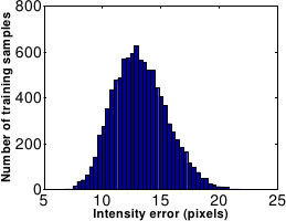
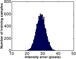
We thus propose to learn a relationship between the intensity error magnitude and displacement magnitude intervals.
We express this relationship in terms of probabilities.
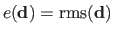
The intensity error magnitude for a residual vector
 is defined as its RMS:
 .
Experimentally, we observed that
.
Experimentally, we observed that
 closely follows a Gaussian distribution, see figure A.24.
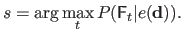
Given the current intensity error
 , finding the most appropriate interaction matrix
 is simply achieved by solving:
 |
(A.47) |
We use an interaction matrix given by:
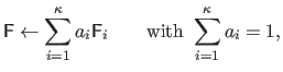 |
(A.48) |
where
 are the mixture proportions.
We compare two mixture models with different probability distributions:
- a Gaussian Mixture Model (GMM):
 , where
follows a Gaussian distribution;
, where
follows a Gaussian distribution;
- a Constant Mixture Model (CMM):
 .
.
For all the piecewise linear relationships described aboveA.6, the interaction matrix
is applied for the last two iterations.
This additional step ensures accuracy.
Experimental Results
We use a simple homographic warp to guarantee a fair comparisonA.7 between the five piecewise linear relationships.
The setup described in section A.6.2.1 is used.
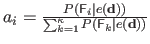
The results are shown in figure A.25.
The five piecewise linear relationships have similar convergence basins.
Their convergence frequency are over  and around
  at a displacement magnitude of 20 pixels and 25 pixels respectively.
CMM seems to have a slightly thiner convergence basin.
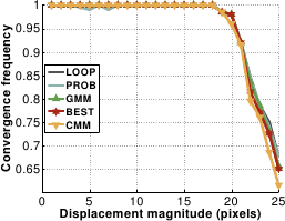
GMM and PROB are quite sensitive to noise.
It corrupts the probability distributions learned off-line.
GMM is slightly better than PROB: at a noise magnitude of
at a displacement magnitude of 20 pixels and 25 pixels respectively.
CMM seems to have a slightly thiner convergence basin.
GMM and PROB are quite sensitive to noise.
It corrupts the probability distributions learned off-line.
GMM is slightly better than PROB: at a noise magnitude of  the convergence frequency of PROB is only
  whereas GMM always converges.
CMM, BEST and LOOP are insensitive to noise.
whereas GMM always converges.
CMM, BEST and LOOP are insensitive to noise.
Figure A.25:
Comparison of the five piecewise linear relationships in terms of convergence frequency against displacement magnitude (a) and noise amplitude (b). On graph (b), CMM and LOOP are indistinguishable.
|
 |
 |
| (a) |
(b) |
|
The results against displacement magnitude are similar for the five piecewise linear relationships.
The associated graph is thus not shown.
The residual error is around 0.025 pixels for all tested magnitudes.
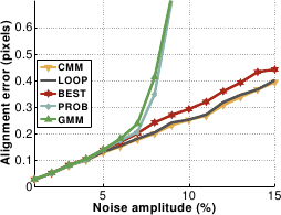
GMM and PROB are less accurate against noise beyond an amplitude of and  respectively than the other piecewise linear relationships.
This is illustrated in figure A.7.2.
Their residual errors are approximately 0.7 pixels against 0.3 pixels for CMM, BEST and LOOP (i.e. , a 2.5 ratio).
respectively than the other piecewise linear relationships.
This is illustrated in figure A.7.2.
Their residual errors are approximately 0.7 pixels against 0.3 pixels for CMM, BEST and LOOP (i.e. , a 2.5 ratio).
Figure A.26:
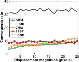
(a) Comparison of the five piecewise linear relationships in terms of convergence rate against displacement magnitude. (b) Comparison of the five piecewise linear relationships in terms of accuracy against noise amplitude.
|
 |
 |
| (a) |
(b) |
|
The results are shown in figure A.7.2.
BEST and LOOP are clearly not efficient against displacement magnitude: LOOP needs at least 30 iterations to converge while BEST requires 10 iterations with high computational cost.
CMM, GMM and PROB do better with a convergence rate kept below 10.
Convergence rates for the five piecewise linear relationships are similar against noise magnitude.
The associated graph is thus not shown.
Overall, CMM is the best piecewise relationship.
It is much more efficient than LOOP and BEST and unaffected by noise contrary to CMM and PROB.
Its convergence basin is only slightly smaller than those induced by the other relationships.
We use the CMM piecewise linear relationship in the experiments of section A.6.2.
Contributions to Parametric Image Registration and 3D Surface Reconstruction (Ph.D. dissertation, November 2010) - Florent Brunet
Webpage generated on July 2011
PDF version (11 Mo)