Subsections
Experimental Results
Representational Similarity of the TPS and FFD Warps
This first set of experiments is designed to compare the TPS and the FFD warp.
In the light of these experiments, we believe that a fair conclusion is that the TPS and the FFD warp have the same order of representational power.
This motivates our choice to only consider the TPS warp in the other experiments of this article.
The experimental setup is as follows.
We synthesize a set of point correspondences
 .
The points
.
The points
 in the first image are taken as the nodes of a regular grid of size
 over the domain
![$ [-1,1] \times [-1,1]$](img1685.png) .
These points are randomly and independently moved (with a given average magnitude
.
These points are randomly and independently moved (with a given average magnitude  ) in order to build the corresponding points
 in the second image.
A TPS and an FFD warp are then estimated from the point correspondences.
The initial data points
and the warped ones are compared using the fitting error defined by:
in the second image.
A TPS and an FFD warp are then estimated from the point correspondences.
The initial data points
and the warped ones are compared using the fitting error defined by:
 |
(A.45) |
where
 represents the estimated warp (either TPS or FFD) and
  the euclidean distance.
Note that the fitting error is expressed in the same unit as the points of the second image.
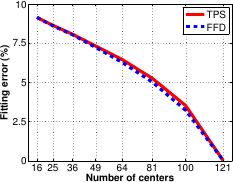
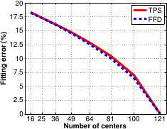
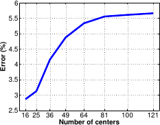
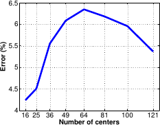
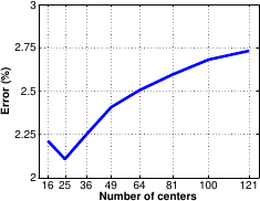
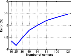
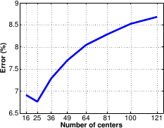
The results are shown in figure A.12 for different displacement magnitudes.
The reported values are obtained as the average over 500 trials.
The fitting errors and the displacement magnitudes are expressed in percentage of the domain size.
We can see that the curves in figure A.12 are almost identical.
It means that none of the two considered warps prevails the other one ;
they can model equally the point correspondences.
Note also that the fitting error collapses to zero when the number of centers is the same as the number of point correspondences.
the euclidean distance.
Note that the fitting error is expressed in the same unit as the points of the second image.
The results are shown in figure A.12 for different displacement magnitudes.
The reported values are obtained as the average over 500 trials.
The fitting errors and the displacement magnitudes are expressed in percentage of the domain size.
We can see that the curves in figure A.12 are almost identical.
It means that none of the two considered warps prevails the other one ;
they can model equally the point correspondences.
Note also that the fitting error collapses to zero when the number of centers is the same as the number of point correspondences.
Figure A.12:
Fitting error between the synthesized data points and the points warped with the estimated TPS and FFD warps ( is the average displacement magnitude.)
|
|
This second experiment differs from the first one in the sense that the point correspondences are not generated randomly.
First, a TPS warp is generated with randomly determined driving features
 .
The centers of this TPS warp are taken on an
.
The centers of this TPS warp are taken on an
 regular grid over the domain
![$ \Omega = [-1,1] \times [-1,1]$](img1691.png) .
The generated driving features
are produced by moving the centers around their initial location with an average magnitude .
Second, a set of point correspondences is synthesized by sampling the TPS warp:
.
The generated driving features
are produced by moving the centers around their initial location with an average magnitude .
Second, a set of point correspondences is synthesized by sampling the TPS warp:
 .
Third, the features
.
Third, the features
 of an FFD warp are determined from the previously generated point correspondences.
Finally, the TPS and the FFD warps are compared using the following measure:
of an FFD warp are determined from the previously generated point correspondences.
Finally, the TPS and the FFD warps are compared using the following measure:
 |
(A.46) |
The unit of this error measure is the same as the one of the points in the second image.
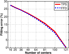
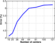
The results are presented in figure A.13.
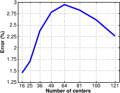
Figure A.14 are the results obtained with the same experimental setup except that the roles of the TPS and the FFD warps have been switched.
The reported errors are computed by averaging over 200 trials.
These errors are expressed in percentage of the domain size.
Figure A.13:
Error between the FFD and the TPS warps. The FFD warp is estimated from point correspondences that comes from the TPS warp ( is the displacement magnitude).
|
|
Figure A.14:
Error between the TPS and the FFD warps. The TPS warp is estimated from point correspondences that come from the FFD warp ( is the displacement magnitude).
|
|
Figure A.13 tells us that given a TPS warp, it is possible to closely approximate the same deformations with an FFD warp. Conversely, the deformations induced by an FFD warp can also be closely approximated by a TPS warp (figure A.14).
Since the parameters in the Feature-Driven framework are meaningful to the warp (i.e. they are interpolated by the warps), we can compare the TPS and the FFD warps with the same set of driving features.
In this experiment, we randomly generate some driving features with their associated centers.
We then compare the TPS and the FFD warps resulting from these features using the same measure as in the previous experiment.
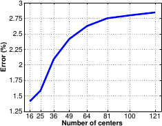
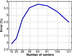
Figure A.15 shows the results for different magnitude of transformation.
The reported numbers are obtained as the average over 200 trials.
Figure A.15:
Comparison of the TPS and of the FFD warps resulting from a common set of driving features ( is the displacement magnitude).
|
|
The values of the errors and the displacement magnitudes in figure A.15 are expressed in percentage of the domain size.
We can see from figure A.15 that TPS and FFD warps induced from the same set of features are close to each other.
Comparison of Registration Algorithms
In this second set of experiments, we compare four algorithms in terms of convergence frequency, accuracy and convergence rate:
- Two classical algorithms:
- FA-GN : the Forward Additive Gauss-Newton approach used by (16,111) and described in section A.2.1.
- FA-ESM : the Efficient Second-order approximation of the cost function proposed by (21) and reviewed in section A.2.1 with an additive update of the parametersA.4.
- Two algorithms we propose:
- IC-GN : the Feature-Driven Inverse Compositional registration of section A.3 with Gauss-Newton as local registration engine as described in section A.4.1.
- FC-LE : the Feature-Driven Forward Compositional registration of section A.3, with local registration achieved through learning as described in section A.4.2.
Simulated Data
In order to assess algorithms in different controlled conditions, we synthesized images from a texture image.
The driving features are placed on a
 grid, randomly perturbed with magnitude
  .
We add Gaussian noise, with variance
.
We add Gaussian noise, with variance  of the maximum greylevel value, to the warped image.
An example of such generated data is shown in figure A.16.
We vary each of these parameters independently, using the following default values:
of the maximum greylevel value, to the warped image.
An example of such generated data is shown in figure A.16.
We vary each of these parameters independently, using the following default values:  pixels and
 .
The estimated warps are scored by the mean Euclidean distance between the driving features which generated the warped image, and the estimated ones.
Convergence to the right solution is declared if this score is lower than one pixel.
The characteristics we measured are:
.
The estimated warps are scored by the mean Euclidean distance between the driving features which generated the warped image, and the estimated ones.
Convergence to the right solution is declared if this score is lower than one pixel.
The characteristics we measured are:
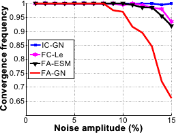
- Convergence frequency.
This is the percentage of convergence to the right solution.
- Accuracy.
This is the mean residual error over the trials for which an algorithm converged.
- Convergence rate.
This is defined by the number of iterations required to converge.
The results are averages over 500 trials.
Note that, in this section, the elements in the legend of each figure are ordered according to their performance (from best to worst).
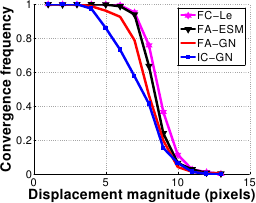
The results are shown in figure A.17.
FC-LE has the largest convergence basin closely followed by FA-ESM.
IC-GN has the smallest convergence basin.
At a displacement magnitude of 8 pixels, the convergence frequency of FC-LE is around 75% whereas it is near only 40% for FA-GN and IC-GN.
FA-GN has the worst performances against noise.
The other algorithms are almost unaffected by noise.
Figure A.17:
Comparison of the four algorithms in terms of convergence frequency against displacement magnitude (a) and noise amplitude (b).
|
 |
 |
| (a) |
(b) |
|
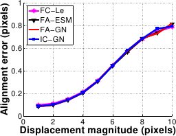
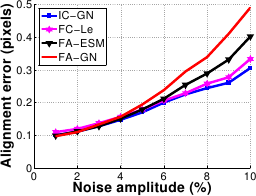
The results are shown in figure A.18.
The four algorithms are equivalent against the displacement magnitude.
Concerning the amplitude of the noise, IC-GN and FC-LE are equivalent while FA-ESM is slightly worse and FA-GN clearly worse.
For example, at 6% noise, the registration errors of IC-GN and FC-LE are around 0.2 pixels, FA-ESM is at about 0.25 pixels and FA-GN at 0.35 pixels.
Figure A.18:
Comparison of the four algorithms in terms of accuracy against displacement magnitude (a) and noise amplitude (b).
|
 |
 |
| (a) |
(b) |
|
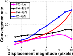
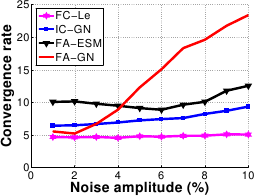
The results are shown in figure A.19.
The convergence rate of FC-LE and FA-ESM are almost constant against both displacement and noise amplitude.
However FC-LE does better, with a convergence rate kept below 10 iterations.
FA-GN and IC-GN are efficient for small displacements, i.e. below 5 pixels.
The convergence rate increases dramatically beyond this value for both of them.
FA-GN is also inefficient for noise amplitude over 4 .
This is explained by the fact that the FA-GN Jacobian matrix depends mainly on the current image gradient, onto which the noise is added.
.
This is explained by the fact that the FA-GN Jacobian matrix depends mainly on the current image gradient, onto which the noise is added.
Figure A.19:
Comparison of the four algorithms in terms of convergence rate against displacement magnitude (a) and noise amplitude (b).
|
 |
 |
| (a) |
(b) |
|
This set of experiments on synthetic data shows that the proposed algorithms, i.e. FC-LE and IC-GN, are always the best ones in the presence of noise.
FC-LE also obtains the best performances against the displacement magnitude.
However, the standard algorithms, i.e. FA-ESM and FA-GN, performs better than IC-GN for important displacement magnitudes.
The four above described algorithms have been compared on several image sequences.
We show results for four such videosA.5.
We measured the average and maximum intensity RMS along the sequence, the total number of iterations and the computational time (expressed in seconds).
The RMS is expressed in pixel value unit.
Note that the RMS is computed on the pixels of interest, i.e. the pixels actually used in the registration algorithms themselves.
All algorithms have been implemented in Matlab.
In order to illustrate the registration, we defined a mesh on the texture image and transferred it to all the other frames.
Note that these meshes are different from the estimated driving features.
The registration differences between the four algorithms are generally visually indistinguishable when they converge.
This sequence has 400 frames.
The displacement magnitude between the frames may be important.
The driving features of the warp are placed on a
grid.
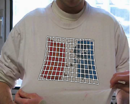
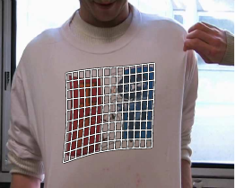
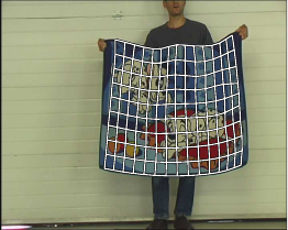
Results are given in table A.3 and registration for the FC-LE algorithm shown in figure A.20.
FC-LE performs well on this sequence.
It is the fastest and the most accurate.
FA-GN, FA-ESM and IC-GN are quite equivalent in terms of alignment accuracy.
FA-GN needs a lot of iterations, making it 5 times slower than FC-LE.
Table A.3:
Results for the first T-shirt sequence. Bold indicates best performances.
|
| |
Mean/max RMS |
# Iteration |
Total/mean time |
|
| FA-GN |
8.70/13.67 |
9057 |
2083/5.2 |
|
| FA-ESM |
9.23/14.77 |
3658 |
877/2.2 |
|
| IC-GN |
9.69/15.82 |
6231 |
436/1.1 |
|
| FC-LE |
6.66/12.87 |
3309 |
380/0.95 |
|
|
Figure A.20:
Registration results for FC-LE on the first T-shirt sequence.
|
|
This sequence has 350 frames.
The driving features of the warp are placed on a
 grid.
The results are given in table A.4 and registration for the FC-LE algorithm shown in figure A.21.
IC-GN diverges when the deformation seems to be the most important.
The other algorithms have similar alignment performances, FA-GN being slightly better.
FC-LE is however 3 times faster than the other algorithms.
grid.
The results are given in table A.4 and registration for the FC-LE algorithm shown in figure A.21.
IC-GN diverges when the deformation seems to be the most important.
The other algorithms have similar alignment performances, FA-GN being slightly better.
FC-LE is however 3 times faster than the other algorithms.
Table A.4:
Results for the paper sequence. The IC-GN algorithm diverges on this sequence. Bold indicates best performances.
|
| |
Mean/max RMS |
# Iteration |
Total/mean time |
|
| FA-GN |
8.98/17.57 |
2422 |
532/1.5 |
|
| FA-ESM |
10.22/20.49 |
2473 |
560/1.6 |
|
| FC-LE |
9.44/19.4 |
1330 |
176/0.5 |
|
|
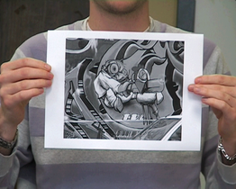
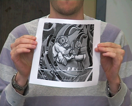
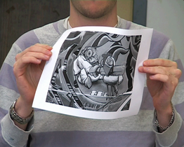
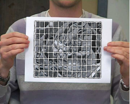
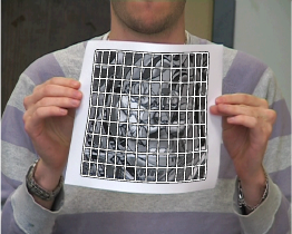
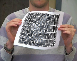
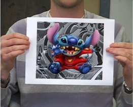
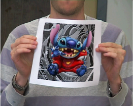
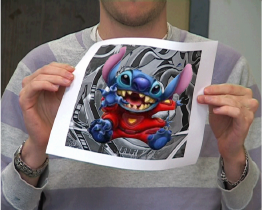
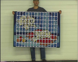
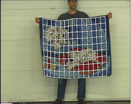
Figure A.21:
First row: the paper sequence. Second row: registration results for FC-LE. Third row: surface augmentation with the Walt Disney character Stitch. Fourth row: deformations are captured and applied on a poster of the Walt Disney movie Cars.
|
|
This short sequence has 42 frames.
The displacement magnitude is high.
The driving features of the warp are placed on a
 grid.
The results are given in table A.5 and registration for the FC-LE algorithm shown in figure A.22.
As for the paper sequence, IC-GN diverges.
FA-GN and FA-ESM give the most accurate alignment, FC-LE being slightly worse.
On the other hand it is 7 times faster.
grid.
The results are given in table A.5 and registration for the FC-LE algorithm shown in figure A.22.
As for the paper sequence, IC-GN diverges.
FA-GN and FA-ESM give the most accurate alignment, FC-LE being slightly worse.
On the other hand it is 7 times faster.
Table A.5:
Results for the rug sequence. The IC-GN algorithm diverges on this sequence. Bold indicates best performances.
|
| |
Mean/max RMS |
# Iteration |
Total/mean time |
| FA-GN |
5.64/8.21 |
538 |
118/2.8 |
| FA-ESM |
5.79/8.63 |
477 |
109/2.6 |
| FC-LE |
6.45/9.80 |
149 |
17.13/0.4 |
|
Figure A.22:
Registration results for FC-LE on the rug sequence.
|
|
This sequence has 623 frames.
Deformations are moderate, but there are strong global illumination variations along the sequence.
The driving features of the warp are placed on a
grid.
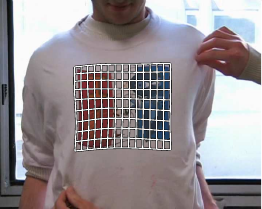
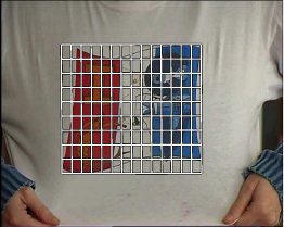
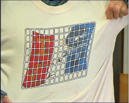
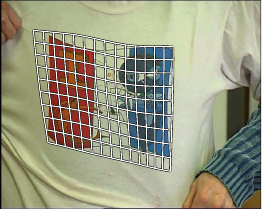
The results are given in table A.6 and registration results for the FC-LE algorithm shown in figure A.23.
The registration is well achieved by the four algorithms.
The small residual error shows that the global illumination changes are correctly compensated.
FC-LE and IC-GN are respectively 4 and 2 times faster than the classical algorithms.
Table A.6:
Results for the second T-shirt sequence. Bold indicates best performances.
|
| |
Mean/max RMS |
# Iteration |
Total/mean time |
|
| FA-GN |
4.51/7.42 |
3408 |
785/1.25 |
|
| FA-ESM |
4.53/7.49 |
3268 |
788/1.25 |
|
| IC-GN |
4.87/7.61 |
4407 |
381/0.61 |
|
| FC-LE |
4.61/7.70 |
1757 |
247/0.39 |
|
|
Figure A.23:
Registration results for FC-LE on the second T-shirt sequence.
|
|
FA-GN is the most accurate algorithm.
It is however inefficient, especially for important displacements.
FA-ESM has almost similar performances compared to the FA-GN while being slightly more efficient.
IC-GN is efficient, but looses effectiveness for high displacements.
As for the experiments with synthetic data, FC-LE has the best behavior: it is similar to FA-GN for accuracy while being 5 times faster on average and is equivalent or better than IC-GN and FA-ESM in terms of alignment accuracy, computational cost and has a larger convergence basin.
Contributions to Parametric Image Registration and 3D Surface Reconstruction (Ph.D. dissertation, November 2010) - Florent Brunet
Webpage generated on July 2011
PDF version (11 Mo)