Subsections
Feature-Driven Warps
In this section, we specialize the generic Feature-Driven parameterization presented in section A.3.1 for two types of warps: the TPS and the FFD warps.
Since the representational power of the TPS warp and of the FFD warp are equivalent (see experiments in section A.6.1), we focused our experiments on the TPS warp.
However, it is important to show how the FFD warp can actually be used in the Feature-Driven framework.
In particular, we show how the standard FFD model can be extended in order to be compatible with the warp reversion operation.
The Feature-Driven Thin-Plate Spline Warp
Ignoring the parameters, a TPS
 is an
is an
 function.
It is the Radial Basis Function that minimizes the integral bending energy.
In its natural parameterization, a TPS is driven by a set of
function.
It is the Radial Basis Function that minimizes the integral bending energy.
In its natural parameterization, a TPS is driven by a set of  weights
 .
These weights are grouped in a vector of parameters
.
These weights are grouped in a vector of parameters
 .
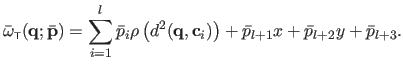
The evaluation of a TPS at the point
.
The evaluation of a TPS at the point
 is given by:
 |
(A.23) |
The  2D points
 are called the centers.
They are also the driving features in the texture image.
They can be located at any place but, in practice, we place them on a regular grid.
The function
are called the centers.
They are also the driving features in the texture image.
They can be located at any place but, in practice, we place them on a regular grid.
The function  gives the squared euclidean distance between its two arguments.
The function
gives the squared euclidean distance between its two arguments.
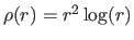
The function  is the TPS basis function and is defined by
 for
for  and
and
 .
In matrix form, equation (A.23) is equivalent to:
.
In matrix form, equation (A.23) is equivalent to:
 |
(A.24) |
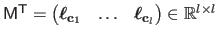
with
 .
.
Standard
 TPS warps are obtained by replacing the scalar weights
  by the control points
 .
The control points are grouped in a single matrix of parameters
.
The control points are grouped in a single matrix of parameters
 defined by
 .
The TPS warp is thus defined by:
.
The TPS warp is thus defined by:
 |
(A.25) |
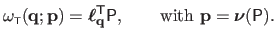
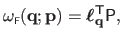
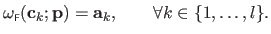
The Feature-Driven parameterization of the TPS warp consists in replacing the control points by some features (i.e. points) in the current image.
A point
 is assigned to each center
defined in the texture image.
The features
is assigned to each center
defined in the texture image.
The features
 are grouped in a single matrix
 .
Similarly, the centers
are grouped in a matrix
.
Similarly, the centers
are grouped in a matrix
 .
Following (24), the control points of a TPS can be determined from the correspondences
.
Following (24), the control points of a TPS can be determined from the correspondences
 :
:
 |
(A.26) |
while enforcing the 3 `side-conditions' ensuring that the TPS has square integrable second derivatives (more details can be found in (193)):
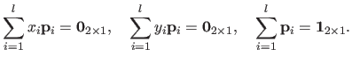 |
(A.27) |
Combining these conditions in a single matrix gives the following exactly determined linear system:
 |
(A.28) |
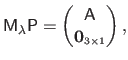
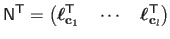
with
 the matrix defined by:
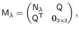 |
(A.29) |
with
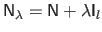 ,
,
 and
and
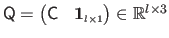 .
Adding
.
Adding
 to
to
 acts as a regularizer.
Determining the control points
acts as a regularizer.
Determining the control points
 from the equation (A.28) can be done in a straightforward manner as the solution of an exactly determined linear system.
The resulting matrix of control points, denoted
from the equation (A.28) can be done in a straightforward manner as the solution of an exactly determined linear system.
The resulting matrix of control points, denoted
 , is a nonlinear function of the regularization parameter
  and a linear function of the features
 :
:
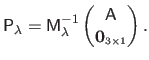 |
(A.30) |
is a linear `back-projection' of the feature matrix
. It can be computed efficiently using the blockwise matrix inversion formulas:
 |
(A.31) |
with:
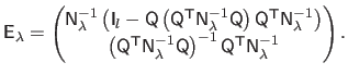 |
(A.32) |
This expression has the advantages of separating and
and introduces units: while
has no obvious unit,
in general has (e.g. pixels, meters).
Finally, if we replace the natural parameters
 in the definition of the TPS warp
 (equation (A.25)) by their expression given in the equation (A.32), we get the Feature-Driven parameterization of the TPS warp, denoted
 :
:
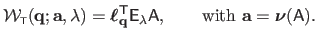 |
(A.33) |
We use the notation
 for
for
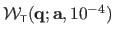 .
We choose
.
We choose
 to ensure good numerical conditioning of the matrix
 .
.
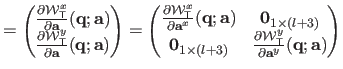
The Jacobian matrix of the warp is needed by the Gauss-Newton based algorithms for local registration (see e.g. , section A.2.1 or section A.4.1).
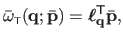
We denote
 the Jacobian matrix of the TPS warp evaluated at the point
 .
It is defined by
.
It is defined by
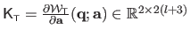 and is given by:
where
 and
and
 are the first and the second coordinates of the warp
and
are the first and the second coordinates of the warp
and
 .
.
The Feature-Driven Free-Form Deformation
Tensor-product B-Splines are a particular model of Free-Form Deformations.
They are a general model of polynomial functions which have been proved to be useful for image registration (162).
Even if there is a wide variety of B-Splines (with various degrees for the polynomial basis or by choosing exotic knot sequences), we limit our study to the case of the Uniform Cubic B-Splines since it best matches the needs of image registration.
For the sake of simplicity, we will abbreviate it FFD.
Ignoring the parameters, a monodimensional FFD
 is an
is an
 function defined as a linear combination of the basis functions
  weighted by the scalars
  called the weights:
 |
(A.35) |
where
 is the vector that contains all the weights .
The basis functions are defined using a knot sequence, i.e. a non-decreasing sequence
is the vector that contains all the weights .
The basis functions are defined using a knot sequence, i.e. a non-decreasing sequence
 . The FFD is said to be uniform when the knot sequence is uniform, i.e. all the knot intervals
![$ [k_i,k_{i+1}]$](img326.png) have the same length
have the same length  .
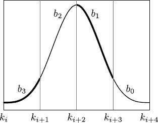
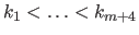
In this case, the basis functions are defined by using four polynomials of degree three, the blending functions (see figure A.8 for an illustration):
.
In this case, the basis functions are defined by using four polynomials of degree three, the blending functions (see figure A.8 for an illustration):
 |
(A.36) |
where  is the normalized abscissa of
  defined as
 for
for
![$ x \in [k_I,k_{I+1}]$](img1627.png) .
.
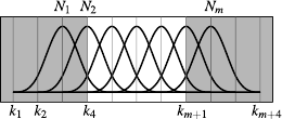
We can see from equation (A.35) that an FFD is non-zero only over the interval
![$ [k_1, k_{m+4}]$](img1628.png) .
However, it is common practice to reduce the domain to
.
However, it is common practice to reduce the domain to
![$ [k_4,k_{m+1}]$](img1629.png) .
By doing so, there are always exactly 4 non-zero basis functions on each knot interval, as figure A.8 illustrates.
.
By doing so, there are always exactly 4 non-zero basis functions on each knot interval, as figure A.8 illustrates.
The standard
FFD warp is obtained as the two-way tensor-product of monodimensional FFD s.
Using its natural parameterization, the evaluation of the FFD warp
 at the point
 is given by:
 |
(A.37) |
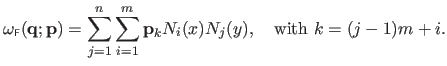
The  control points
 are grouped in the vector
 that is defined as
 where
where
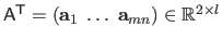
 is the matrix given by
 .
The control points of an FFD warp are not more meaningful than the ones of a TPS warp.
They are not interpolated: they just act as `attractors' to the warp.
Equation (A.37) can be rewritten in matrix form:
.
The control points of an FFD warp are not more meaningful than the ones of a TPS warp.
They are not interpolated: they just act as `attractors' to the warp.
Equation (A.37) can be rewritten in matrix form:
 |
(A.38) |
where
 is the vector defined by:
 |
(A.39) |
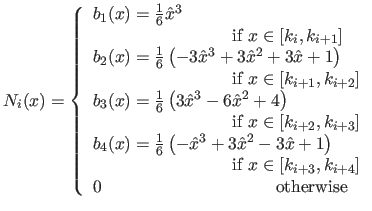
The Feature-Driven parameterization of the FFD warp is similar to the one of the TPS warp in the sense that it makes the warp driven by features expressed in pixels in both the texture and the current images.
The centers of the TPS warp were used as features in the texture image.
Such centers do not exist for FFD warps.
We thus introduce a set of points
that will be used as features in the texture image.
We call these points centers for consistency with the TPS warps.
We use  centers located on a regular grid.
A feature
in the current image is associated to every center
.
The control points
of the FFD warp can be determined from the correspondences
by enforcing the following constraints:
centers located on a regular grid.
A feature
in the current image is associated to every center
.
The control points
of the FFD warp can be determined from the correspondences
by enforcing the following constraints:
 |
(A.40) |
Since the number of features is equal to the number of degrees of freedom of the FFD warp, the determination of the parameters from the features can be carried out with an exactly determined linear system:
 |
(A.41) |
with
 ,
,
 and
and
 .
The solution of the linear system of equation (A.41) can be written
.
The solution of the linear system of equation (A.41) can be written
 where
where
 .
The existence of the matrix
.
The existence of the matrix
 is guaranteed if the Schoenberg-Whitney conditions are satisfied (see (57)) as it is the case when the centers are located on a regular grid.
Note that the matrix
can be pre-computed.
Finally, the Feature-Driven parameterization of the FFD warp, denoted
is guaranteed if the Schoenberg-Whitney conditions are satisfied (see (57)) as it is the case when the centers are located on a regular grid.
Note that the matrix
can be pre-computed.
Finally, the Feature-Driven parameterization of the FFD warp, denoted
 , is given by replacing the natural parameters
in equation (A.38) with their expression in function of the features
, is given by replacing the natural parameters
in equation (A.38) with their expression in function of the features
 :
:
 |
(A.42) |
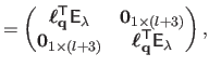
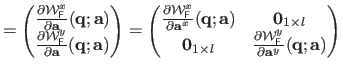
The Jacobian matrix
 for FFD warps can be computed following exactly the same reasoning as for the TPS warp:
The computations involved in the warp reversion operation (see section A.3.3) can lead to evaluate a warp outside of its natural definition domain.
More precisely, in equation (A.11), nothing ensures that the features of the vector
 lies in the domain of the warp.
While this is not a problem with the TPS warp whose domain is infinite, extra work need to be done with the FFD warp.
Indeed, with the previous definition, it is possible to evaluate an FFD warp outside of its natural domain but it is meaningless since it collapses to 0.
In this section, we propose a new method to extrapolate an FFD warp outside of its domain making it virtually infinite.
lies in the domain of the warp.
While this is not a problem with the TPS warp whose domain is infinite, extra work need to be done with the FFD warp.
Indeed, with the previous definition, it is possible to evaluate an FFD warp outside of its natural domain but it is meaningless since it collapses to 0.
In this section, we propose a new method to extrapolate an FFD warp outside of its domain making it virtually infinite.
The principle of the method is simple:
a linear extension is added to the basis that crosses the boundaries of the domain (with some extra conditions of continuity and differentiability).
While this seems almost trivial in the monodimensional case, it is less simple in two dimensions, i.e. for warps.
Our strategy consists in defining the extension in 1D and, then, propagate it to the 2D case using the usual tensor-product.
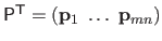
We present the extrapolation approach in the monodimensional case and for the leftmost boundary of the domain (i.e. , the knot  ).
The four non-zero bases that cross this boundary are
).
The four non-zero bases that cross this boundary are  ,
,  ,
,  and
and  .
Our idea is to drop the part of these bases that are outside the domain and to replace them with a linear extension.
We call
.
Our idea is to drop the part of these bases that are outside the domain and to replace them with a linear extension.
We call  ,
,  ,
,  and
and  the bases resulting from this process.
In addition to be linear, we enforce the following constraints in order to preserve continuity and differentiability:
the bases resulting from this process.
In addition to be linear, we enforce the following constraints in order to preserve continuity and differentiability:
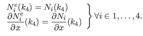 |
(A.44) |
For the sake of simplicity and without loss of generality, we consider that the leftmost boundary coincides with zero ( ) and that the length of the knot intervals is consistently one (
 ).
Under all these constraints, it follows that:
).
Under all these constraints, it follows that:
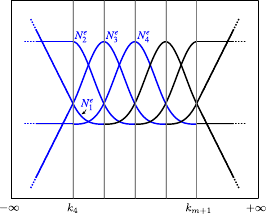
The extended basis for the rightmost boundary are obtained by symmetry.
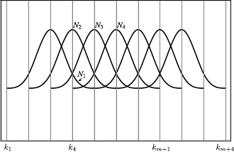
Figure A.9 illustrates the resulting extended basis functions.
The twodimensional counterparts of these newly defined extended basis functions are obtained using the tensor-product.
Figure A.9:
(a) Standard basis functions. (b) Extended basis functions that allow one to extrapolate outside the natural domain
.
|
|
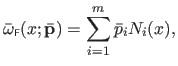
The proposed extension gives a remarkably good behavior to the extrapolating functions.
See figure A.10 and figure A.11 for an illustration in 1D and 2D respectively.
Besides, the fact that the basis functions form a partition of unity remains true (
![$ \sum_{i=1}^4 N_i^e(x) = 1, \forall x \in (-\infty,0]$](img1681.png) ).
).
Figure A.10:
Examples of our extrapolating FFD in the monodimensional case. The extrapolating parts are represented with dashed lines.
|
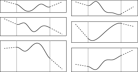 |
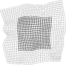
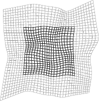
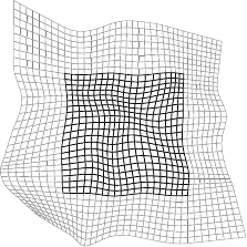
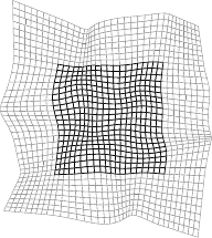
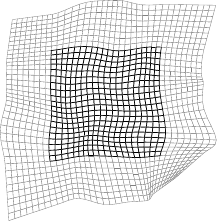
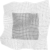
Figure A.11:
Examples of our extrapolating FFD warp. The dark part of the meshes represents the warp over its initial domain while the light part is extrapolated.
|
|
Contributions to Parametric Image Registration and 3D Surface Reconstruction (Ph.D. dissertation, November 2010) - Florent Brunet
Webpage generated on July 2011
PDF version (11 Mo)
![$\displaystyle =
\begin{cases}
\displaystyle -\frac{x}{2}+\frac{1}{6} & \textrm{if $x \in (-\infty, 0]$}
N_1(x) & \textrm{otherwise}
\end{cases}$](img1674.png)
![$\displaystyle =
\begin{cases}
\displaystyle \frac{2}{3} & \textrm{if $x \in (-\infty, 0]$}
N_2(x) & \textrm{otherwise}
\end{cases}$](img1676.png)
![$\displaystyle =
\begin{cases}
\displaystyle \frac{x}{2}+\frac{1}{6} & \textrm{if $x \in (-\infty, 0]$}
N_3(x) & \textrm{otherwise}
\end{cases}$](img1678.png)
![$\displaystyle =
\begin{cases}
\displaystyle 0 & \textrm{if $x \in (-\infty, 0]$}
N_4(x) & \textrm{otherwise}
\end{cases}$](img1680.png)