Subsections
Local Registration Algorithms
In the literature, there are two ways for estimating local registration: the Forward and the Inverse approaches (9).
The former evaluates directly the warp which aligns the texture image
 with the warped image
 .
The latter computes the warp which aligns the warped with the texture image and then inverts the warp.
They are both compatible with approximations of the cost function such as Gauss-Newton, ESM, learning-based, etc
We describe in details the Inverse Gauss-Newton and the Forward Learning-based local registration steps.
.
The latter computes the warp which aligns the warped with the texture image and then inverts the warp.
They are both compatible with approximations of the cost function such as Gauss-Newton, ESM, learning-based, etc
We describe in details the Inverse Gauss-Newton and the Forward Learning-based local registration steps.
Local Registration with Gauss-Newton
Combining an Inverse local registration with a Gauss-Newton approximation of the cost function is efficient since this combination makes invariant the approximated Hessian matrix used in the normal equations to be solved at each iteration.
We cast this approach in the Feature-Driven framework, making it possible to extend Inverse Compositional registration to the TPS and the FFD warps.
In the Inverse Compositional framework, local registration is achieved by minimizing the local discrepancy error:
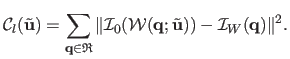 |
(A.16) |
Using Gauss-Newton as local registration engine, the gradient vector is the product of the texture image gradient vector and of the constant Jacobian matrix
 of the warp:
 .
Matrix
is given in section A.5.
The Jacobian matrix of this least squares cost is thus constant.
The Hessian matrix
.
Matrix
is given in section A.5.
The Jacobian matrix of this least squares cost is thus constant.
The Hessian matrix
 and its inverse are computed off-line.
However, the driving features
and its inverse are computed off-line.
However, the driving features
 are located on the reference image
.
They must be located on the warped image
for being used in the update.
We use our warp reversion process for finding the driving features
are located on the reference image
.
They must be located on the warped image
for being used in the update.
We use our warp reversion process for finding the driving features
 on the warped image i.e. ,
such that
on the warped image i.e. ,
such that
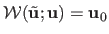 .
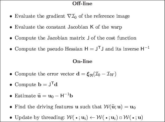
An overview of Feature-Driven Inverse Gauss-Newton registration is shown in table A.1.
.
An overview of Feature-Driven Inverse Gauss-Newton registration is shown in table A.1.
Table A.1:
Overview of our Feature-Driven Inverse Compositional Gauss-Newton registration.
 |
Learning-Based Local Registration
Learning-based methods model the relationship between the local increment
 and the intensity discrepancy
 with an interaction function
  :
:
 |
(A.17) |
The interaction function is often approximated using a linear model, i.e.
 where
where
 is called the interaction matrix.
This relationship is valid locally around the texture image parameters
is called the interaction matrix.
This relationship is valid locally around the texture image parameters
 .
Compositional algorithms are thus required, as in (104) for homographic warps.
The Feature-Driven framework naturally extends this approach to non-groupwise warps.
However in (49) the assumption is made that the domain where the linear relationship is valid covers the whole set of registrations.
They thus apply their interaction function around the current parameters, avoiding the warping and the composition steps.
This does not appear to be a valid choice in practice.
.
Compositional algorithms are thus required, as in (104) for homographic warps.
The Feature-Driven framework naturally extends this approach to non-groupwise warps.
However in (49) the assumption is made that the domain where the linear relationship is valid covers the whole set of registrations.
They thus apply their interaction function around the current parameters, avoiding the warping and the composition steps.
This does not appear to be a valid choice in practice.
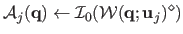
The interaction function is learned from artificially perturbed texture images
 .
They are obtained through random perturbations of the reference parameter
.
In the literature, linear and non linear interaction functions are used.
They are learned with different regression algorithms such as Least Squares (LS) (104,49), Support Vector Machines (SVM) or Relevance Vector Machines (RVM) (1).
Details are given below for a linear interaction function, i.e. an interaction matrix, learned through Least Squares regression.
Table A.2 summarizes the steps of learning-based local registration.
.
They are obtained through random perturbations of the reference parameter
.
In the literature, linear and non linear interaction functions are used.
They are learned with different regression algorithms such as Least Squares (LS) (104,49), Support Vector Machines (SVM) or Relevance Vector Machines (RVM) (1).
Details are given below for a linear interaction function, i.e. an interaction matrix, learned through Least Squares regression.
Table A.2 summarizes the steps of learning-based local registration.
Table A.2:
Overview of our Learning-based registration.
|
The driving features in the texture image are disturbed from their rest position
with randomly chosen directions
 and magnitudes
 :
:
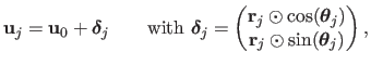 |
(A.18) |
where
 and
and
 are meant to be applied to all the elements of
and
are meant to be applied to all the elements of
and  denotes the element-wise product.
The magnitude is clamped between a lower and an upper bound, determining the area of validity of the interaction matrix to be learned.
For a Feature-Driven warp, fixing this magnitude is straightforward since the driving features are expressed in pixels.
It can be much more complex when the parameters are difficult to interpret such as the usual coefficients of the TPS and the FFD warps.
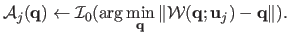
There are two ways to synthesize images:
denotes the element-wise product.
The magnitude is clamped between a lower and an upper bound, determining the area of validity of the interaction matrix to be learned.
For a Feature-Driven warp, fixing this magnitude is straightforward since the driving features are expressed in pixels.
It can be much more complex when the parameters are difficult to interpret such as the usual coefficients of the TPS and the FFD warps.
There are two ways to synthesize images:
| |
|
 |
(A.19) |
| |
|
or |
|
| |
|
 |
(A.20) |
The former requires warp inversion whereas the latter requires a cost optimization, per-pixel. In our experiments, we use equation (A.19).
Our Feature-Driven warp reversion process is thus used to warp the texture image.
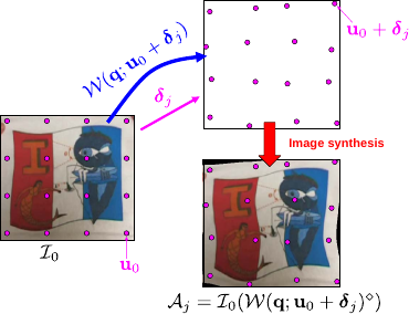
Training data generation with a Feature-Driven warp is illustrated in figure A.7.
Figure A.7:
Generating training data with a Feature-Driven warp.
|
 |
The residual vector is computed for the pixels of interest in
 :
:
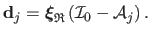 |
(A.21) |
The training data are gathered in matrices
 and
and
 .
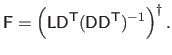
The interaction matrix
.
The interaction matrix
 is computed by minimizing a Linear Least Squares error in the image space, expressed in pixel value unit, giving:
 |
(A.22) |
This is one of the two possibilities for learning the interaction matrix.
The other possibility is dual. It minimizes an error in the parameter space, i.e. expressed in pixels.
The two approaches have been experimentally compared. Learning the interaction matrix in the image space give the best results.
Thereafter, we use this option.
Experiments show that a linear approximation of the relationship between the local increment
and the intensity discrepancy
, though computationally efficient, does not always give satisfying results.
The drawback is that if the interaction matrix covers a large domain of deformation magnitudes, the registration accuracy is spoiled.
On the other hand, if the matrix is learned for small deformations only, the convergence basin is dramatically reduced.
Using a nonlinear interaction function learned through RVM or SVM partially solves this issue.
We use a simple piecewise linear relationship as interaction function.
It means that we learn not only one but a series
 of interaction matrices, each of them covering a different range of displacement magnitudes.
The interaction function is thus of the form
of interaction matrices, each of them covering a different range of displacement magnitudes.
The interaction function is thus of the form
 .
More details are given in appendix A.7.
.
More details are given in appendix A.7.
Contributions to Parametric Image Registration and 3D Surface Reconstruction (Ph.D. dissertation, November 2010) - Florent Brunet
Webpage generated on July 2011
PDF version (11 Mo)