Subsections
Feature-Driven Registration
In this section, we present our principal contribution: the Feature-Driven framework.
This framework, in which one directly acts on warp driving features, has two main advantages.
First, it often is better balanced to tune feature positions, expressed in pixels, than coefficient vectors that may be difficult to interpret, as for the TPS or the FFD warps.
Second, it allows one to use the efficient compositional framework in a straightforward manner.
Indeed, warp composition and inversion cannot be directly done for non-groupwise warps.
We propose empirical means for approximating warp composition and inversion through their driving features, called threading and reversion respectively.
Our Feature-Driven framework is generic in the sense that it can be applied to almost any parametric warps such as the TPS or the FFD warps, as shown in section A.5.
Feature-Driven Warp Parameterization
Ignoring the set of parameters, a warp is an
 function usually parameterized by a set of
  control points
 for
for
 .
These control points are grouped in a vector
.
These control points are grouped in a vector
 where
where
 is the matrix defined by
 .
We write
.
We write  the warp in its natural parameterization.
The warp is said to be linear when it can be defined as a linear combination of its control points:
the warp in its natural parameterization.
The warp is said to be linear when it can be defined as a linear combination of its control points:
 |
(A.8) |
where
 is a vector that depends on the point
 and on the type of warp being considered.
Note that the dependency on
of
and on the type of warp being considered.
Note that the dependency on
of
 is usually non linear even if the warp is linear.
The control points are usually not interpolated.
They just act as `attractors' to the warp.
It thus makes their interpretation difficult.
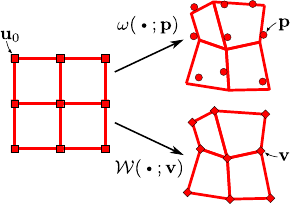
The Feature-Driven concept is in fact a change of parameterization.
The control points are replaced by a set of features that are interpolated by the warp.
We call them the driving features and denote them
is usually non linear even if the warp is linear.
The control points are usually not interpolated.
They just act as `attractors' to the warp.
It thus makes their interpretation difficult.
The Feature-Driven concept is in fact a change of parameterization.
The control points are replaced by a set of features that are interpolated by the warp.
We call them the driving features and denote them
 in the texture image and
 in the current one (see figure A.1).
We denote
in the current one (see figure A.1).
We denote
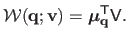
 the Feature-Driven parameterization of the warp .
Loosely speaking, matching the driving features between two images is equivalent to defining a warp since the warp can be used to transfer the driving features from one image to the other, while conversely, the warp can be computed from the driving features.
Indeed, if the warp is linear with respect to its control points then it is always possible to find a matrix
the Feature-Driven parameterization of the warp .
Loosely speaking, matching the driving features between two images is equivalent to defining a warp since the warp can be used to transfer the driving features from one image to the other, while conversely, the warp can be computed from the driving features.
Indeed, if the warp is linear with respect to its control points then it is always possible to find a matrix
 such that:
 |
(A.9) |
with
 , i.e.
 equals to
reshaped on two columns.
Matrix
can be pre-computed.
Details on how the matrix
is obtained for the TPS and the FFD warps are given in section A.5.1 and section A.5.2 respectively.
If we write
equals to
reshaped on two columns.
Matrix
can be pre-computed.
Details on how the matrix
is obtained for the TPS and the FFD warps are given in section A.5.1 and section A.5.2 respectively.
If we write
 then the Feature-Driven parameterization of the warp
is given by:
then the Feature-Driven parameterization of the warp
is given by:
 |
(A.10) |
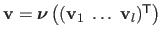
If we denote
the features in the texture image then
 is the identity warpA.3, i.e. the warp that leaves the location of the features
unchanged.
is the identity warpA.3, i.e. the warp that leaves the location of the features
unchanged.
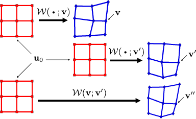
Given two sets of driving features,
 and
and
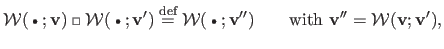
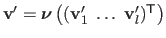 , we want to find a third set
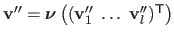 defined such that threading the warps induced by
and
defined such that threading the warps induced by
and
 results in the warp induced by
 , as shown in figure A.2.
We propose a simple and computationally cheap way to do it, as opposed to previous work.
This is possible thanks to the Feature-Driven parameterization.
Our idea for threading warps is very simple: we apply the
induced warp to the features
; the resulting set of features is
.
We thus define the warp threading operator, denoted
, as shown in figure A.2.
We propose a simple and computationally cheap way to do it, as opposed to previous work.
This is possible thanks to the Feature-Driven parameterization.
Our idea for threading warps is very simple: we apply the
induced warp to the features
; the resulting set of features is
.
We thus define the warp threading operator, denoted
 , as:
, as:
 |
(A.11) |
where
 is meant to be applied to each feature in
.
is meant to be applied to each feature in
.
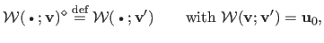
Examples of our warp threading process are shown in figure A.3.
We synthesized two sets of driving features
and
by randomly disturbing a
 regular grid from its rest position
.
As expected, threading a warp
regular grid from its rest position
.
As expected, threading a warp
 with the identity
returns the original warp i.e.
with the identity
returns the original warp i.e.
 and
and
 .
.
Figure A.3:
Examples for the warp threading process.
|
 |
Reverting Warps
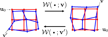
Given a set
of driving features, we want to determine the features
such that the warp they induce is the reversion of the one induced by
.
This is illustrated in figure A.4.
As for the threading, our Feature-Driven framework yields a very simple solution.
The idea is that applying the
induced warp to
should give
i.e. , the fixed driving features in the texture image.
We thus introduce the reversion operator  as:
as:
 |
(A.12) |
This amounts to solving an exactly determined linear system, the size of which is the number of driving features.
Using equation (A.10), we obtain:
 |
(A.13) |
where
 is the matrix defined by
 ,
,
 and
and
 .
The driving features
of the reverted warp are thus given by:
.
The driving features
of the reverted warp are thus given by:
 |
(A.14) |
Examples of the reverting process are shown in figure A.5.
We synthesized driving features
by randomly disturbing a
regular grid from its rest position
.
The driving features
result from reverting the warp
.
Threading warps
and
 introduce a new set of driving features
.
As expected, the features
are similar to the original grid
with an average residual error of
introduce a new set of driving features
.
As expected, the features
are similar to the original grid
with an average residual error of  pixels.
Figure A.5:
Illustration of the warp reversion process on three examples.
|
 |
Relying on the Feature-Driven parameterization properties, we extend compositional algorithms to non-groupwise warps.
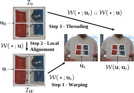
The following three steps are repeated until convergence, as shown in figure A.6:
Note that in previous work (158,75,123) a preliminary step is required before applying the update rule, as reviewed in section A.2.2.
In comparison, our Feature-Driven framework makes it naturally included into the third step.
Illumination changes are handled by globally normalizing the pixel values in the texture and the warped images at each iteration.
Another approach could be used such as the light-invariant approach of (148).
Figure A.6:
The three steps of the Compositional Feature-Driven registration.
|
 |
Contributions to Parametric Image Registration and 3D Surface Reconstruction (Ph.D. dissertation, November 2010) - Florent Brunet
Webpage generated on July 2011
PDF version (11 Mo)