Subsections
Pixel-Based Hyperparameter Selection for Feature-Based Image Registration
In this section, we deal with parametric image registration from point correspondences in deformable environments.
In this problem, it is essential to determine correct values for hyperparameters such as the number of control points of the warp, a smoothing parameter weighting a term in the cost function, or an M-estimator threshold.
This is usually carried out either manually by a trial-and-error procedure or automatically by optimizing a criterion such as the Cross-Validation score (see section 3.2.2).
In this section, we propose a new criterion that makes use of all the available image photometric information.
We use the point correspondences as a training set to determine the warp parameters and the photometric information as a test set to tune the hyperparameters.
Our approach is fully robust in the sense that it copes with both erroneous point correspondences and outliers in the images caused by, for instance, occlusions or specularities.
Parametric image registration is the problem of finding the (natural) parameters of a warp such that it aligns a source image to a target image.
In addition to these natural parameters, one also has to determine correct values for the problem hyperparameters in order to get a proper registration.
The hyperparameters are either additional parameters of the warp itself (warp hyperparameters) or parameters included in the cost function to optimize (cost hyperparameters).
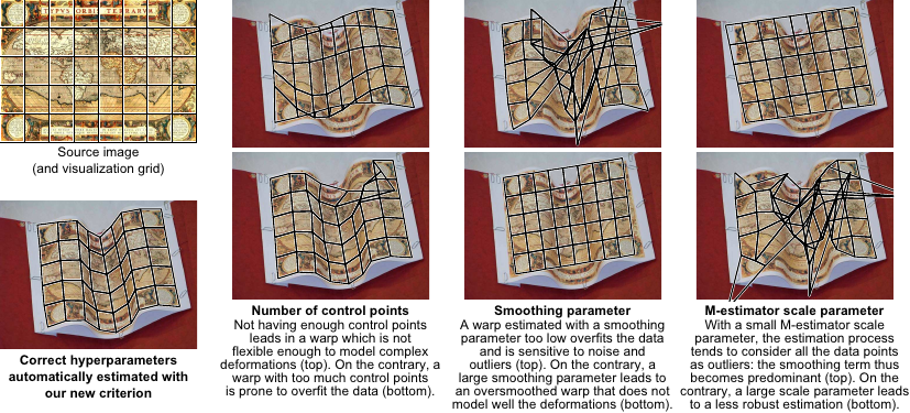
As illustrated in figure 5.17, the hyperparameters greatly influence the quality of the estimated warp.
As reviewed previously, there are two main approaches to image registration: the feature-based and the pixel-based (or direct) approaches.
They both have their own drawbacks and advantages but neither of them directly enables one to automatically tune the hyperparameters.
In this section, we propose a new method to automatically set the hyperparameters by combining the advantages of the feature-based and the pixel-based approaches.
As just said, some hyperparameters are linked to the warp.
Let
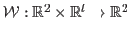 be a warp.
It is primarily parametrized by a set of
be a warp.
It is primarily parametrized by a set of  parameters arranged in a vector
 .
The homography (94,181) is an example of warp, often parametrized by the 8 independent coefficients of the homography matrix.
Another example of warp is the Free-Form Deformation (FFD) (162) parametrized by
.
The homography (94,181) is an example of warp, often parametrized by the 8 independent coefficients of the homography matrix.
Another example of warp is the Free-Form Deformation (FFD) (162) parametrized by  two-dimensional control points.
Examples of hyperparameters linked to the warps include, but are not limited to, the number of control points of an FFD or the kernel bandwidth of a Radial Basis Function (24).
two-dimensional control points.
Examples of hyperparameters linked to the warps include, but are not limited to, the number of control points of an FFD or the kernel bandwidth of a Radial Basis Function (24).
Figure 5.17:
Illustration of how some typical hyperparameters influence image registration. The contribution of this paper is a method able to select the proper hyperparameters by combining the advantages of the feature-based and of the pixel-based approaches to image registration. In this example, the data points were automatically detected and matched with SIFT (115,190). There was approximately 200 point correspondences (not shown in the figure) uniformly spread across the source image. Among these points, around 10% were gross outliers.
|
 |
In this section, we use a slightly different formalism than the one used in the introductory section of this chapter.
This is motivated by the fact that we now explicitly consider the hyperparameters bundled in the feature-based approach to image registration.
Let
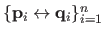 be the point correspondences.
We now write the optimization problem of the feature-based image registration as:
be the point correspondences.
We now write the optimization problem of the feature-based image registration as:
 |
(5.23) |
where
 is a vector containing all the hyperparameters and
 is the vector of the natural parameters of the warp.
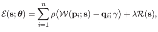
 is the cost function that may be defined as, for instance:
 |
(5.24) |
with  an M-estimator,
  its scale parameter,
 a smoothing term such as the classical bending energy term discussed in section 5.1.2.1 (equation (5.11)) and
  a smoothing term controlling the trade-off between goodness-of-fit and smoothing.
In equation (5.24), and are two examples of cost hyperparameters.
Note that other hyperparameters can appear in the cost function if one decides, for instance, to use more terms.
The main advantages of the feature-based approach to image registration are that it copes with large deformations and it is efficient in terms of computational complexity (this is particularly true when using an efficient keypoint detector such as SIFT (115) or SURF (20) combined with a good matching algorithm such as the improved nearest neighbour algorithm suggested in (115) and implemented in (190)).
However, the feature-based approach by itself does not enable one to determine correct hyperparameters.
It is not possible to determine proper values for the hyperparameters by including them directly in the optimization problem (5.23), i.e.
a smoothing term controlling the trade-off between goodness-of-fit and smoothing.
In equation (5.24), and are two examples of cost hyperparameters.
Note that other hyperparameters can appear in the cost function if one decides, for instance, to use more terms.
The main advantages of the feature-based approach to image registration are that it copes with large deformations and it is efficient in terms of computational complexity (this is particularly true when using an efficient keypoint detector such as SIFT (115) or SURF (20) combined with a good matching algorithm such as the improved nearest neighbour algorithm suggested in (115) and implemented in (190)).
However, the feature-based approach by itself does not enable one to determine correct hyperparameters.
It is not possible to determine proper values for the hyperparameters by including them directly in the optimization problem (5.23), i.e.
 .
This comes from the general arguments that were developed in section 3.2.
.
This comes from the general arguments that were developed in section 3.2.
The other approach to image registration is the direct approach (9,101).
In this case, the warp parameters are estimated by minimizing the pixel-wise dissimilarities between the source image and the warped target image.
One advantage of this approach is that the data used for the parameter estimation is denser than with the feature-based approach.
As in the feature-based approach, it is not possible to estimate the hyperparameters with the direct approach.
Since the hyperparameters cannot be trivially estimated, they are often fixed once and for all according to some empirical (and often unreliable) observations.
It is also possible to choose them manually with some kind of trial-and-error procedure.
This technique is obviously not satisfactory because of its lack of automatism and of foundations.
Several approaches have been proposed to tune the hyperparameters in an automatic way.
None of them is specific to image registration.
They generally minimize a criterion that depends on the hyperparameters and that assesses the `quality' of the estimated parameters by measuring the ability of the current estimate to generalize to new data.
They include, but are not limited to, Akaike Information Criterion (45), Mallow's  (160), Minimum Description Length criterion, and the techniques relying on Cross-Validation scores (27,194,12).
These types of approach were reviewed in section 3.2.2.
(160), Minimum Description Length criterion, and the techniques relying on Cross-Validation scores (27,194,12).
These types of approach were reviewed in section 3.2.2.
The common characteristic of these approaches to automatically select the hyperparameters is that they are problem generic and, as a consequence, they all rely on the point correspondences only.
In the particular context of feature-based image registration, another type of data is available: the photometric information.
We thus propose a new criterion, named the photometric criterion, that uses the point correspondences as a training set and the pixel colours as a test set.
Another way to put it is to say that our approach combines the two classical approaches to image registration: roughly speaking, the feature-based approach is used to estimate the natural parameters while the pixel-based approach is used for the hyperparameters.
Our photometric criterion is more flexible than the previous approaches in the sense that it can handle simultaneously several hyperparameters of different types (for instance, discrete and continuous hyperparameters can be mixed together).
Besides, our approach is much more robust to erroneous data (noise and outliers) than previous approaches based on Cross-Validation.
Also, it still works when there are only a few point correspondences.
Our new criterion is explained in section 5.3.3 and its ability to properly tune several hyperparameters simultaneously is experimented in section 5.3.4 with B-spline warps and the Cauchy M-estimator.
Reminder and Complementary Elements on Automatic Hyperparameter Selection
We presented several hyperparameters in the introduction of this section.
It is important to understand that inconsistent results would arise if one tries to estimate the hyperparameters by including them in the optimization problem (5.23).
For instance, with such an approach, the best way to minimize the contribution of the regularization term would be to set
 which is obviously not the desired value.
All the same way, making the M-estimator scale parameter tend to 0 would `artificially' decrease the value of the cost function because it would be equivalent to consider that almost all the point correspondences are outliers (and the cost assigned to outliers tends to zero when
which is obviously not the desired value.
All the same way, making the M-estimator scale parameter tend to 0 would `artificially' decrease the value of the cost function because it would be equivalent to consider that almost all the point correspondences are outliers (and the cost assigned to outliers tends to zero when
 ).
).
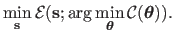
As we explained in section 3.2, the classical approach to build an automatic procedure for selecting the hyperparameters consists in designing a criterion
 that assesses the `quality' of a given set of hyperparameters (193,12).
The minimizer of this criterion should be the set of hyperparameters to use.
The complete problem thus consists in solving the following nested optimization problem:
that assesses the `quality' of a given set of hyperparameters (193,12).
The minimizer of this criterion should be the set of hyperparameters to use.
The complete problem thus consists in solving the following nested optimization problem:
 |
(5.25) |
Note that the introduction of the criterion
makes the problem (5.25) completely different from the inconsistent problem
.
Cross-Validation
Cross-Validation (hereinafter abbreviated CV) is a general principle used to tune the hyperparameters in parameter estimation problems (193).
Broadly speaking, a CV procedure consists in minimizing a score function that measures how well a set of estimated parameters will generalize to new data.
This is achieved by dividing the whole data set into several subsets.
Each one of these subsets is then alternatively used as a training set or as a test set to build the CV score function.
The use of CV to select the hyperparameters for spline parameter estimation has been introduced in (194).
It has been successfully applied for deformable warp estimation from point correspondences in (12).
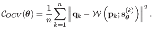
We now give a reminder of two variants of CV which allow us to fix the notation used in this section: the Ordinary CV and the  -fold CV .
For a given set of hyperparameters
, let
 be the warp parameters estimated from the data with the
  -th point correspondence left out.
The OCV score, denoted
-th point correspondence left out.
The OCV score, denoted
 , is defined by:
 |
(5.26) |
Tuning the hyperparameters using the OCV consists in minimizing
with respect to
.
This approach has several drawbacks.
First, computing
is prohibitive: evaluating
for a single
with equation (5.26) requires to estimate each one of the  vectors
 .
There exists some close approximations of equation (5.26) resulting in a significant improvement in terms of computational time.
However, these approximations are only usable in a least-squares framework for parameter estimation (see, for instance, (66,11)).
Second, the score
is not robust to false point correspondences.
And last, but not least, the OCV score is not reliable when there are not enough point correspondences (193).
.
There exists some close approximations of equation (5.26) resulting in a significant improvement in terms of computational time.
However, these approximations are only usable in a least-squares framework for parameter estimation (see, for instance, (66,11)).
Second, the score
is not robust to false point correspondences.
And last, but not least, the OCV score is not reliable when there are not enough point correspondences (193).
An alternative to the OCV score is the -fold CV score.
A complete review of the -fold CV is given in (27).
It consists in splitting the set of point correspondences into disjoint sets of nearly equal sizes (with usually chosen as
 ).
Let
).
Let
![$ \mathbf{s}_{\mathbold{\theta}}^{[v]}$](img1219.png) be the warp parameters obtained from the data with the
be the warp parameters obtained from the data with the  -th group left out and let
  be the number of point correspondences in the -th group.
The -fold CV score, denoted
be the number of point correspondences in the -th group.
The -fold CV score, denoted
 , is defined by:
![$\displaystyle \mathcal {C}_{V}(\mathbold{\theta}) = \sum_{v=1}^V \frac{m_v}{n} ...
...eft( \mathbf{p}_k ; \mathbf{s}_{\mathbold{\theta}}^{[v]} \right) \right\Vert^2.$](img1221.png) |
(5.27) |
The -fold CV is not robust to erroneous point correspondences.
It can be made robust by replacing the average
![$ \sum_{k=1}^{m_v} \frac{1}{m_v} \left\Vert \mathbf{q}_k - \mathcal {W} \left( \mathbf{p}_k ; \mathbf{s}_{\mathbold{\theta}}^{[v]} \right) \right\Vert^2$](img1222.png) in equation (5.27) with some robust measure such as the trimmed mean (27).
Besides, the -fold CV score is not more reliable than the OCV score when there are only a few point correspondences.
in equation (5.27) with some robust measure such as the trimmed mean (27).
Besides, the -fold CV score is not more reliable than the OCV score when there are only a few point correspondences.
Other approaches such as Akaike Information Criterion (AIC), Bayesian Information Criterion (BIC), Mallow's , Minimum Description Length (MDL) have been used to tune hyperparameters (see, for instance, (45,27)).
Some robust versions also exist for these criteria ; for instance a robust Mallow's is developed in (160).
However, these criteria have usually been developed to choose one model among a finite set of given models and, as such, approaches based on CV are better suited to tune continuous hyperparameters (12).
Our Contribution: the Photometric Error Criterion
The common characteristic of the approaches reviewed in section 3.2.2 is that both the parameters and the hyperparameters are estimated using exactly the same data set, i.e. the point correspondences.
In this section, we propose a new criterion to tune hyperparameters that makes use of all the available information: not only the point correspondences but also the photometric information.
The principle of our approach consists in combining the two standard approaches to image registration:
- given a set of hyperparameters
, the feature-based approach is used to determine the warp parameters
 from the point correspondences ;
- the cost function of the direct approach is used to assess the correctness of the hyperparameters
: the proper hyperparameters must be the ones minimizing the pixel-wise photometric discrepancy between the target image and the warped source image.
In other words, we propose to use the point correspondences as the training set and the photometric information as the test set.
Dividing the data into a training set and a test set is a classical approach of statistical learning (96).
Given a vector of hyperparameters
and the corresponding warp parameters
(estimated from the point correspondences), our criterion, denoted
 , is defined as:
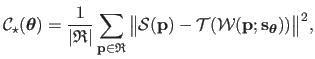 |
(5.28) |
where
 is the region of interest and
 its size.
can be defined as, for instance, a rectangle obtained by cropping the domain of the source image.
More advanced techniques such as the one proposed in the previous section could also be used to deal with the region of interest.
However, since the region of interest is not the central point of this section, we prefer to keep it as simple as possible.
its size.
can be defined as, for instance, a rectangle obtained by cropping the domain of the source image.
More advanced techniques such as the one proposed in the previous section could also be used to deal with the region of interest.
However, since the region of interest is not the central point of this section, we prefer to keep it as simple as possible.
Note that the criterion of equation (5.28) is a slight variation of the cost function typically minimized in direct image registration (101,181) (see section 5.1.2.1).
The only difference is the normalizing factor
 .
This factor allows one to compensate the undesirable effects due to the overlap problem (see section 5.2).
Using this factor in classical direct image registration would make difficult the optimization process since it makes the cost function non-linear with respect to the warp parameters.
However, in the context now considered, the criterion of equation (5.28) is not intended to be minimized with respect to the warp parameters.
This is the very difference with direct image registration: here, the criterion of equation (5.28) is considered as a function of the hyperparameters
, not of the warp parameters
.
.
This factor allows one to compensate the undesirable effects due to the overlap problem (see section 5.2).
Using this factor in classical direct image registration would make difficult the optimization process since it makes the cost function non-linear with respect to the warp parameters.
However, in the context now considered, the criterion of equation (5.28) is not intended to be minimized with respect to the warp parameters.
This is the very difference with direct image registration: here, the criterion of equation (5.28) is considered as a function of the hyperparameters
, not of the warp parameters
.
When using photometric information, one should take care of the fact that there can be outliers in the image colours caused, for instance, by occlusions or specularities.
The criterion
can be made robust to these outliers by replacing the squared Euclidean norm in equation (5.28) with a more robust measure such as the trimmed mean.
We thus define the robust photometric error criterion, denoted
 , as:
, as:
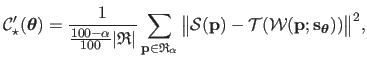 |
(5.29) |
where
 is the subset of
obtained by removing from
the
is the subset of
obtained by removing from
the  of the pixels that produce the highest values for
 (see section 3.1.2.3).
Experimental Results
The contribution we presented in this section is quite generic in the sense that it may be used in many different setup.
However, even though our contribution is generic, we use a particular combination of elements for the experiments of this section.
We use the uniform cubic B-spline model of function for the warp (see section 2.3.2.3 and section 2.3.2.5).
This model is interesting since it is generic and may thus represent the transformations of a deformable environment.
Besides, this model includes several hyperparameters.
The number of control points is one of these hyperparameters (we note this number in the sequel of the experiments).
In order to compute a smooth warp, we use the classical bending energy term as described in section 5.1.2.1 (equation (5.11)).
Using such a regularization scheme introduce another hyperparameter: the regularization parameter, which we denote in the rest of the experiments.
In this section we use the Cauchy M-estimator defined by the following function:
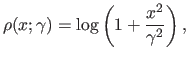 |
(5.30) |
where
 is an hyperparameter that controls the scale of this M-estimator.
More details on this M-estimator may be found in section 3.1.2.2.
In particular, it can easily be shown that the Cauchy M-estimator is the negative likelihood with errors following a Cauchy/Lorentz distribution.
The inaccuracies of the keypoints' locations detected by SURF and SIFT tend to follow such a distribution.
Besides, the probability density function (PDF) of the Cauchy distribution has heavy tails that satisfactorily models the outliers, i.e. the false point correspondences.
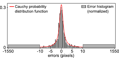
We report in figure 5.18 an illustrative test showing that assuming a Cauchy distribution is consistent with the kind of errors encountered in real cases.
In this experiment, we use the source and the target images of figure 5.17 for which the ground truth warp is known (manually determined).
Figure 5.18 depicts an histogram of the errors between the location of the 1112 keypoints detected with SIFT in the target image and their expected location (computed by applying the ground truth warp to the keypoints in the source image).
It shows that considering a Cauchy distribution is a reasonable choice.
In particular, the fact that the tails of the PDF of the Cauchy distribution are heavier than the ones of, for instance, the Gaussian PDF makes the cost function of equation (5.23) robust to outliers.
is an hyperparameter that controls the scale of this M-estimator.
More details on this M-estimator may be found in section 3.1.2.2.
In particular, it can easily be shown that the Cauchy M-estimator is the negative likelihood with errors following a Cauchy/Lorentz distribution.
The inaccuracies of the keypoints' locations detected by SURF and SIFT tend to follow such a distribution.
Besides, the probability density function (PDF) of the Cauchy distribution has heavy tails that satisfactorily models the outliers, i.e. the false point correspondences.
We report in figure 5.18 an illustrative test showing that assuming a Cauchy distribution is consistent with the kind of errors encountered in real cases.
In this experiment, we use the source and the target images of figure 5.17 for which the ground truth warp is known (manually determined).
Figure 5.18 depicts an histogram of the errors between the location of the 1112 keypoints detected with SIFT in the target image and their expected location (computed by applying the ground truth warp to the keypoints in the source image).
It shows that considering a Cauchy distribution is a reasonable choice.
In particular, the fact that the tails of the PDF of the Cauchy distribution are heavier than the ones of, for instance, the Gaussian PDF makes the cost function of equation (5.23) robust to outliers.
Figure 5.18:
Graphical comparison between the probability density function of the Cauchy distribution and the (normalized) histogram of the errors between the expected keypoints in the target image and the keypoints automatically detected with SIFT. Mind the scale of the abscissa axis.
|
 |
All the criteria used in the experiments (including the CV criteria and our new criterion) are minimized using an exhaustive search approach.
It consists in evaluating the criteria over a fine grid in order to find the optimum.
Although long to compute, this approach has the advantage of being reliable.
Besides, we generally optimize over only 2 or 3 hyperparameters, which makes the computational time reasonable.
Synthetic Data
In this subsection, several experiments are done on synthetic data.
Using such data is interesting since it allows us to know precisely the ground truth warp that relates the source and the target images.
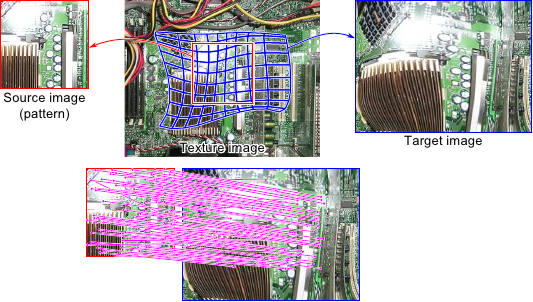
A pair of images is generated from a texture image (randomly chosen in a stock of 15 different images).
A rectangular part of the texture image is used as the source image.
The target image is build by deforming another part of the texture image with a ground truth warp
 , as illustrated in figure 5.19.
The warp
is a B-spline with
, as illustrated in figure 5.19.
The warp
is a B-spline with
 control points determined randomly and such that the average deformation magnitude is approximately 20 pixels.
The sizes of the source and of the target images are
control points determined randomly and such that the average deformation magnitude is approximately 20 pixels.
The sizes of the source and of the target images are
 pixels and
 pixels respectively.
A Gaussian noise with standard deviation equal to
pixels respectively.
A Gaussian noise with standard deviation equal to  of the maximal intensity value is added to the pixels of both the source and the target images.
A set
of the maximal intensity value is added to the pixels of both the source and the target images.
A set
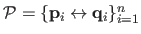 of point correspondences is built by randomly picking the points
 in the source image and computing their correspondents
 in the target image with the warp
.
A Cauchy noise with scale parameter
in the target image with the warp
.
A Cauchy noise with scale parameter
 pixel is added to the point correspondences.
Figure 5.19:
Illustration of the generation of synthetic data. First row: a pair of images (the source and the target images) are generated from a texture image using a predetermined warp (used as the ground truth warp). Second row: point correspondences are automatically extracted and matched from the generated images using standard approaches such as SIFT and SURF.
|
 |
We call oracle the warp estimated from the point correspondences
 which is as close as possible to the ground truth warp
.
It is designed to be the best possible warp given i) the available data and ii) the warp model.
It is preferable to use the oracle instead of the ground truth warp to evaluate an estimated warp.
Indeed, en error between an estimated warp and the ground truth warp does not necessarily comes from a bad estimation process (which is the object of our experiments in this paper): it can comes from the fact that the considered warp model is simply not able to fit the ground truth warp (for example, even if the correct hyperparameters are given, a homography will never fit a highly deformed warp).
The oracle is defined as the warp induced by the parameters and the hyperparameters
which is as close as possible to the ground truth warp
.
It is designed to be the best possible warp given i) the available data and ii) the warp model.
It is preferable to use the oracle instead of the ground truth warp to evaluate an estimated warp.
Indeed, en error between an estimated warp and the ground truth warp does not necessarily comes from a bad estimation process (which is the object of our experiments in this paper): it can comes from the fact that the considered warp model is simply not able to fit the ground truth warp (for example, even if the correct hyperparameters are given, a homography will never fit a highly deformed warp).
The oracle is defined as the warp induced by the parameters and the hyperparameters
 estimated by solving the following problem:
 |
(5.31) |
Problem (5.31) is numerically solved using an exhaustive search approach.
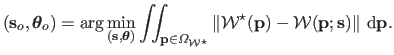
Relative Geometric Error (RGE)
The RGE measures the discrepancy between an estimated warp and the oracle.
Let
 be the set of hyperparameters that minimizes the criterion
 .
Let
.
Let
 be the warp parameters estimated from the point correspondences with the hyperparameters
.
The RGE is defined as:
be the warp parameters estimated from the point correspondences with the hyperparameters
.
The RGE is defined as:
 |
(5.32) |
Figure 5.20 compares the RGE obtained by tuning the M-estimator scale parameter and the smoothing parameter with different approaches:
- our photometric criterion (Photo) and its robust versions with thresholds for the trimmed mean of
 (PhotoR25) and
  (PhotoR50) ;
- the -fold CV criterion (VFold) and its robust versions with thresholds for the trimmed mean of
 (VFoldR20) and
  (VFoldR40).
The number of control points of the warp is set to
 .
100 point correspondences are used to estimate the warp.
The results reported in figure 5.20 are averaged over 100 trials (with different texture images, different point correspondences, and different deformations).
.
100 point correspondences are used to estimate the warp.
The results reported in figure 5.20 are averaged over 100 trials (with different texture images, different point correspondences, and different deformations).
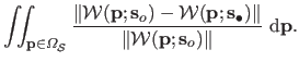
We can observe in figure 5.20 that the smallest RGE are consistently obtained with our photometric criterion.
The difference between robust and non-robust versions of our criterion is not as significant as for the CV criteria.
This comes from the fact that in the synthetic data used for this experiment, there are outliers in the point correspondences (thus affecting the non-robust CV scores) while the source and the target images are outlier-free.
Figure 5.20:
Relative geometric errors for several criteria used to determine hyperparameters. Globally, the criteria we propose (Photo, PhotoR25, and PhotoR50) give better results than the ones obtained with criteria relying on Cross-Validation (VFold, VFoldR20, and VFoldR40). The red line is the median over the 100 trials. The limits of the blue box are the 25th and the 75th percentiles. The black `whiskers' cover approximately 99.3% of the experiment outcomes. The red crosses are the outcomes considered as outliers.
|
|
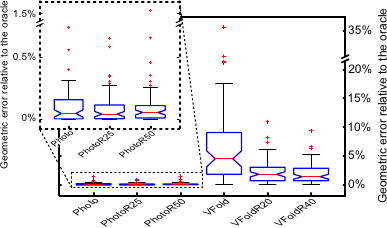
Figure 5.21 shows the values determined with several criteria for the Cauchy's M-estimator scale parameter .
In addition to the criteria used in the previous experiment, we also show the results obtained with the oracle.
The data used in this experiment are the same than the one used in the previous experiment.
The point correspondences were generated with errors following a Cauchy distribution with scale parameter equals to 1.
As a consequence, the criteria are expected to give the value 1 for the scale parameter of the Cauchy's M-estimator.
Figure 5.21 shows that the proposed photometric criteria results in values for which are close to 1.
We observe that the three approaches based on the basic -fold CV also results in correct values.
On the contrary, the robust variants of the -fold CV gives values farther away from 1 than the other approaches.
The fact that the value 1 is not exactly retrieved with our criteria is not really significant since this value is not precisely retrieved with the oracle itself.
Figure 5.21:
Scale parameter of the Cauchy's M-estimator retrieved using several criteria. The pink dashed line represents the expected value for this hyperparameter. The green dashed line represents the value retrieved using the oracle. The use of the criteria we proposed (Photo, PhotoR25, and PhotoR50) results in values close to the expected ones.
|
 |
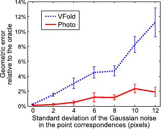
In this experiment, we study the influence of the noise in the point correspondences.
We use the same data than in the experiments of section 5.3.4.3 except that there are no outliers in the images.
The point correspondences are perturbed using an additive Gaussian noise of standard deviation  varying between 0 and 12 pixels.
Therefore, we only test the non-robust methods: VFold and Photo.
These methods are used to automatically tune the regularization parameter.
Figure 5.22 shows the evolution of the RGE in function of the amount of noise in the point correspondences.
It shows that our approach Photo is much more robust to the noise than VFold.
This comes from the fact that VFold entirely relies on the noisy point correspondences while our approach also includes colour information.
varying between 0 and 12 pixels.
Therefore, we only test the non-robust methods: VFold and Photo.
These methods are used to automatically tune the regularization parameter.
Figure 5.22 shows the evolution of the RGE in function of the amount of noise in the point correspondences.
It shows that our approach Photo is much more robust to the noise than VFold.
This comes from the fact that VFold entirely relies on the noisy point correspondences while our approach also includes colour information.
Figure 5.22:
Evolution of the relative geometric error in function of the (Gaussian) noise in the point correspondences. Our approach, Photo, is more robust than the approach relying on the CV (VFold).
|
 |
The last experiments of this paper are conducted on real data.
The source images are digital pictures.
The target images are obtained by first printing the source images and second picturing them with a standard camera.
Ground truth warps were determined manually by clicking several hundreds of point correspondences in the images.
Note that figure 5.17 shows an example of our approach applied to real data.
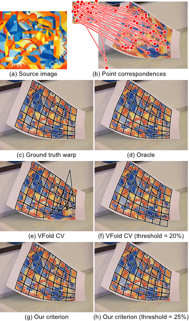
Figure 5.23 shows the registration results obtained by automatically determining the hyperparameters with several criteria.
In this experiment, three hyperparameters were considered: the smoothing parameter , the M-estimator threshold , and the number of control points of the B-spline warp  (the number of control points along the x-axis and the y-axis were set to be equal).
314 point correspondences were automatically determined using the SIFT detector and the descriptor matcher implemented in (190).
Approximately 8% of the point correspondences were false matches.
We can observe in figure 5.23 that our photometric criterion is the one giving the best results.
The standard V-Fold CV criterion is the one leading to the worst results due to the presence of erroneous point correspondences.
The robust V-Fold CV criterion performs better than the non-robust one but is not as good as ours, particularly for the bottom right corner of the image: this is due to a lack of point correspondences in this part of the image.
(the number of control points along the x-axis and the y-axis were set to be equal).
314 point correspondences were automatically determined using the SIFT detector and the descriptor matcher implemented in (190).
Approximately 8% of the point correspondences were false matches.
We can observe in figure 5.23 that our photometric criterion is the one giving the best results.
The standard V-Fold CV criterion is the one leading to the worst results due to the presence of erroneous point correspondences.
The robust V-Fold CV criterion performs better than the non-robust one but is not as good as ours, particularly for the bottom right corner of the image: this is due to a lack of point correspondences in this part of the image.
We report in table 5.2 the RGE as defined in section 5.3.4.3 for the warps estimated in the `cubist image' experiment.
Table 5.2:
RGE for the experiment of figure 5.23.
|
|
Criterion |
RGE |
|
V-Fold CV |
1.852% |
|
V-Fold CV (robust) |
0.675% |
|
Our criterion |
0.190% |
|
Our criterion (robust variant) |
0.197% |
|
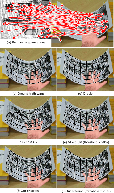
Figure 5.24 shows an experiment similar to the one conducted with the `cubist image'.
Nonetheless, there are some important differences.
This time, the keypoints were extracted using the SURF detector of (20) and approximately 12% of the 621 point correspondences were erroneous.
An artificial occlusion was added to the target image; we used an artificial occlusion in order to still be able to determine the ground truth warp (which is done before the insertion of the occlusion).
Besides, the M-estimator scale parameter and the smoothing parameter were the only hyperparameters under study (the number of control points of the warp was set to the one of the ground truth warp).
As in the `cubist image' case, the hyperparameters chosen with our photometric criterion are better than the ones estimated with the criterion relying on the V-Fold Cross-Validation.
In both cases, the robust versions of the criteria perform better than the non-robust ones.
Note that the occlusion added to the target image influences the non-robust V-fold CV criterion since it introduces supplementary false point correspondences.
Conclusion
We proposed a new criterion to automatically tune the hyperparameters in image registration problems.
We showed that our photometric criterion performs generally better than other approaches with similar goals such as the Cross-Validation criteria.
This was made possible by designing a criterion specifically adapted to the image registration problem that combines the advantages of both the feature-based and the direct approaches to image registration.
Our criterion was successfully experimented in a particular but challenging setup: deformable B-spline warps, selection of an M-estimator threshold, presence of outliers and occlusions, etc.
However, the proposed criterion is not limited to this setup: it is generic enough to be applied in other image registration problems with different constraints, different warps, and, thus, different hyperparameters.
Contributions to Parametric Image Registration and 3D Surface Reconstruction (Ph.D. dissertation, November 2010) - Florent Brunet
Webpage generated on July 2011
PDF version (11 Mo)